Batched, Multi-Dimensional Gaussian Process Regression with GPyTorch

Hands-on Tutorials

Kriging [1], more generally known as Gaussian Process Regression (GPR), is a powerful, non-parametric Bayesian regression technique that can be used for applications ranging from time series forecasting to interpolation.

GPyTorch [2], a package designed for Gaussian Processes, leverages significant advancements in hardware acceleration through a PyTorch backend, batched training and inference, and hardware acceleration through CUDA.

In this article, we look into a specific application of GPyTorch: Fitting Gaussian Process Regression models for batched, multidimensional interpolation.

Imports and Requirements

Before we get started, let’s make sure all packages are installed and imported.

Installation Block

To use GPyTorch for inference, you’ll need to install gpytorch and pytorch:

# Alternatively, you can install pytorch with conda
pip install gyptorch pytorch numpy matplotlib scikit-learn

Import Block

Once our packages have been installed, we can import all our needed packages:

# GPyTorch Imports
import gpytorch
from gpytorch.models import ExactGP, IndependentModelList
from gpytorch.means import ConstantMean, MultitaskMean
from gpytorch.kernels import ScaleKernel, MultitaskKernel
from gpytorch.kernels import RBFKernel, RBFKernel, ProductKernel
from gpytorch.likelihoods import GaussianLikelihood, LikelihoodList, MultitaskGaussianLikelihood
from gpytorch.mlls import SumMarginalLogLikelihood, ExactMarginalLogLikelihood
from gpytorch.distributions import MultivariateNormal, MultitaskMultivariateNormal

# PyTorch
import torch

# Math, avoiding memory leak, and timing
import math
import gc
import math

Creating a Batched GPyTorch Model

To create a batched model, and more generally any model in GPyTorch, we subclass the gpytorch.models.ExactGP class. Like standard PyTorch models, we only need to define the constructor and forward methods for this class. For this demo, we consider two classes, one with a kernel over our entire input space, and one with a factored kernel [5] over our different inputs.

Full Input, Batched Model:

This model computes a kernel between all dimensions of the input, using an RBF/Squared Exponential Kernel that is wrapped with an outputscale hyperparameter. Additionally, you have the option of using Automatic Relevance Determination (ARD) [2] for creating one lengthscale parameter for each feature dimension.

Factored Kernel Model:

This model computes a factored kernel between all dimensions of the input, using a product of RBF/Squared Exponential Kernels that each consider separate dimensions of the feature space. This factored, product kernel is then wrapped with an outputscale hyperparameter. Additionally, you have the option of using Automatic Relevance Determination (ARD) [2] for creating one lengthscale parameter for each feature dimension in both of the RBF kernels.

Preprocessing Data

To prepare data for fitting the Gaussian Process Regressor, it is helpful to consider how our models will be fit. To take advantage of hardware acceleration and batching with PyTorch [3] and CUDA [4], we will model each outcome of our predicted set of variables as independent.

Therefore, if we have B batches of data we need to fit for interpolation, each with N samples with an X-dimension of C and a Y-dimension of D, then we map our datasets into the following dimensions:

1. *X-data: (B, N, C) → (B D, N, C) … This is accomplished via tiling.**
2. *Y-data: (B, N, D) →(B D, N) … This is accomplished via stacking.**

In a sense, we tile our X-dimensional data such that the features are repeated D times for each value our vector-valued Y takes. This means that each model in our set of batched models will be responsible for learning a mapping between the features of one batch of X and a single output feature in the same batch of Y, ** resulting in a total of B * D** models in our batched model. This preprocessing (tiling and stacking) is accomplished via the following code block:

# Preprocess batch data
B, N, XD = Zs.shape
YD = Ys.shape[-1]
batch_shape = B * YD

if use_cuda:  # If GPU available
    output_device = torch.device('cuda:0')  # GPU

# Format the training features - tile and reshape
train_x = torch.tensor(Zs, device=output_device)
train_x = train_x.repeat((YD, 1, 1))

# Format the training labels - reshape
train_y = torch.vstack(
    [torch.tensor(Ys, device=output_device)[..., i] for i in range(YD)])

# train_x.shape
# --> (B*D, N, C)
# train_y.shape
# --> (B*D, N)

We perform these transformations because although GPyTorch has frameworks designed for batched models and multidimensional models (denoted multitask in the package documentation), unfortunately (to the best of my knowledge) GPyTorch does not yet support batched, multidimensional models. The code above trades not being able to model the correlations between the different dimensions of Y for a large improvement in runtime due to batching and hardware acceleration.

Training Batched, Multidimensional GPR Models!

Now, with our model created and our data preprocessed, we are ready to train! The script below performs this training for optimizing hyperparameters using PyTorch’s automatic differentiation framework. In this case, the following batched hyperparameters are optimized:

1. Lengthscale
2. Outputscale
3. Covariance Noise (Raw and Constrained)

Please take a look at this page [5] for more information about the role of each of these hyperparameters.

This training function is given below:

Running Inference

Now that we have trained a set of batched, multidimensional Gaussian Process Regression models on our training data, we are now ready to run inference, in this case, for interpolation.

To demonstrate the efficacy of this fitting, we will be training a batched, multidimensional model and comparing its predictions to an analytic sine function evaluated on randomly-generated data, i.e.

X = {xi}, xi ~ N(0_d, I_d), i.i.d.

Y = sin(X), element-wise, i.e. yi = sin(xi) for all i

(Where 0_d and I_d refer to the d-dimensional zero-vector (zero mean) and d-dimensional identity matrix (identity covariance). The X and Y above will serve as our test data.

To evaluate the quality of these predictions, we will compute the Root Mean Squared Error (RMSE) of our resulting predictions compared to the true analytic value of Y. For this, we will sample one test point per batch (C dimensions in X, and D dimensions in Y), i.e. each GPR model we fit in our batched GPR model will predict a single outcome. The RMSE will be computed across the predicted samples for all batches.

Results

The above experiment results in an average RMSE across batches of approximately 0.01. Try it yourself!

Below are results generated from the script above, showing the predicted vs. true values for each dimension in X and Y:

Below is a table with RMSE values averaged over 10 iterations for different degrees of variance of the underlying data distribution:

Summary

In this article, we saw that we can create batched, multi-dimensional Gaussian Process Regression models using GPyTorch, a state-of-the-art library that leverages PyTorch on its backend for accelerated inference and optimization.

We evaluated this batched, multi-dimensional Gaussian Process Regression model using an experiment with analytic sine waves, and found that we were able to achieve an RMSE of approximately 0.01 when regressing on multivariate, i.i.d, standard normal-generated data, showing that the non-parametric power of these models is highly suitable for a variety of function approximation and regression tasks.

Stay tuned for a full GitHub repository!

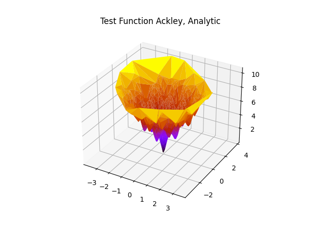
Here are more visualizations! Note that the models below leverage a batch size of 1, but are derived from the same class as the models above and learn a one-dimensional Gaussian Process Regressor for each output dimension.

References

[1] Oliver, Margaret A., and Richard Webster. "Kriging: a method of interpolation for geographical information systems." International Journal of Geographical Information System 4.3 (1990): 313–332.

[2] Gardner, Jacob R., et al. "Gpytorch: Blackbox matrix-matrix gaussian process inference with gpu acceleration." arXiv preprint arXiv:1809.11165 (2018).

[3] Adam Paszke, Sam Gross, Francisco Massa, Adam Lerer, James Bradbury, Gregory Chanan, Trevor Killeen, Zeming Lin, Natalia Gimelshein, Luca Antiga, Alban Desmaison, Andreas Kopf, Edward Yang, Zachary DeVito, Martin Raison, Alykhan Tejani, Sasank Chilamkurthy, Benoit Steiner, Lu Fang, Junjie Bai, and Soumith Chintala. Pytorch: An imperative style, high-performance deep learning library. In H. Wallach, H. Larochelle, A. Beygelzimer, F. dAlché-Buc, E. Fox, and R. Garnett, editors, Advances in Neural Information Processing Systems 32, pages 8024–8035. Curran Associates, Inc., 2019.

[4] NVIDIA, Vingelmann, P., & Fitzek, F. H. P. (2020). CUDA, release: 10.2.89. Retrieved from https://developer.nvidia.com/cuda-toolkit.

[5] Kernel Cookbook, https://www.cs.toronto.edu/~duvenaud/cookbook/.