Causal Effects

This article is a continuation of a 3-part series **** on causality. Previous posts focused on causal inference and causal discovery. This post builds upon these ideas and describes three different causal effects. In future posts, we will discuss computing causal effects from observational data and evaluating causal effects using the do-operator.

Key Point:

Causal effects quantify the impact of a treatment by comparing the outcomes of different treatment values

Why?

The notion of cause and effect plays a central role in how we (i.e. humans) understand the world around us. For example, "the sidewalk is wet because it rained last night", enables us to make inferences in new situations, e.g. why is the patio furniture wet?

This comes down to a fundamental question, why? Why did this happen? What is the cause of this? Or, where is this going? What will be the effect?

In many practical settings (e.g. business, healthcare, education) it is not only advantageous to know what caused what, but by how much? In other words, what degree of the patio furniture’s wetness is due to the rain from last night versus the sprinklers from this morning? Answering this question of "how much?" is what causal effects are all about.

Background

Before diving into how we can answer this question of "how much?", we need to define some things. Those who are familiar with these concepts can feel free to jump to the next section.

Outcomes, Treatments, and Covariates

A key distinction we must make is between the variables available in the study, namely: outcomes, treatments, and covariates.

An outcome is the variable in which we are ultimately interested. For a business, it might be profit, for a clinician it could be the incidence of heart disease, etc.

Treatments are the variables we want to change in order to influence the outcome variable. For example, a business might want to change ad spend to influence profit, or a clinician might change dosages to influence the incidence of heart disease.

Then there are covariates, which are basically everything else. For the clinical example, this could be: age, weight, height, are they a smoker?, exercise level, etc. Throughout this series, outcomes will be represented by Y, treatments by X, and covariates by Z.

Potential Outcomes Framework

A big idea in causality is the Potential Outcomes Framework, which is an approach to estimating causal effects. This framework is built on a core question. Consider a subject in the context of a Randomized Controlled Trial (RCT), what value would the outcome variable (Y) be if the subject had received one treatment (X=x_1) in lieu of another (X=x_0).

This is an example of a counterfactual question i.e. what if A happened instead of B? The fundamental challenge with this question is that each subject can only ever receive one treatment. For example, if I take a Tylenol and my headache goes away, there is no way to observe what would have happened if I didn’t take the pill.

Although we can never truly observe counterfactuals (i.e. what would happen if I received treatment A instead of B), this theoretical concept is a good starting point for a discussion of causal effects.

3 Types of Causal Effects

Here, I describe 3 different types of causal effects. While the expressions provided consider boolean treatments (e.g. take the pill or not), these can be generalized to any number of treatment levels.

1) Individual Treatment Effect (ITE)

Visual breakdown of an individual treatment effect (ITE). Image by author.

An individual treatment effect (ITE) quantifies the impact of treatment for a particular individual. It does this by comparing outcomes for different levels of treatment. This is just like the Tylenol example from before.

In one scenario, I take a Tylenol and my headache goes away. Then suppose, in the counterfactual scenario (i.e. if I didn’t take the pill) my headache wouldn’t go away, but I felt a little better. To evaluate the ITE for this scenario we would compare the pill outcome to the no-pill outcome.

One way to express this is given in the image below.

A way to express individual treatment effects (ITEs). Image by author.

Where, Y(1) represents the outcome value for the pill scenario (i.e. X=1) and Y(0) represents the outcome of the no-pill scenario (i.e. X=0). I will emphasize again, that in reality, we can only observe one of the two scenarios in the ITE equation. Therefore, ITEs are (at best) something we estimate, but never measure directly, and even this can be challenging. The challenge is that ITEs ask for a lot, i.e. what is the treatment effect for a particular individual, at a particular time, in a particular context?

An alternative approach is to expand our population. Then, we can indeed evaluate the treatment effects at a particular time and context, but just not for a particular individual. We would instead obtain population-level treatment effects, which brings us to the 2nd type of causal effect.

2) Average Treatment Effect (ATE)

Visual breakdown of an average treatment effect (ATE). Image by author.

As mentioned before, a problem with ITEs is that they can never truly be measured. But, what if we turned our aim to population-level effects? This is exactly what the Average Treatment Effect (ATE) quantifies. In other words, an ATE estimates the expected impact of treatment for a population. Just like the ITE, it works by comparing outcomes for different levels of treatment. However, instead of considering a particular individual, it evaluates a whole population.

This can be expressed as follows:

A way to express average treatment effects (ATEs) [1]. Image by author.

Where E{V} represents the expectation value (i.e. average) of some variable V. _Yi(1) represents the ith subject’s outcome value for the pill scenario. And, _Yi(0) represents the ith subject’s outcome value for the no-pill scenario. What makes the ATE much easier to estimate is the expectation value. Meaning, we are interested in averages, not point estimates.

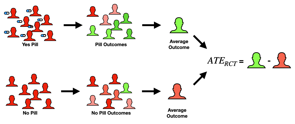
This is one of the most prominent ways to quantify treatment effects. It commonly appears in the context of Randomized Controlled Trials (RCTs), where the whole population is randomly split into 2 equal groups (e.g. pill and no pill groups). It is very important that the splitting be done at random and equal groups so that for a sufficiently large population size, the 2 groups are directly comparable. This then reduces the ATE equation from before into something very easy to compute (see below expression).

Average treatment effect (ATE) in a Randomized Controlled Trial (RCT) [1]. Image by author.

Where j indexes the treatment group and k indexes the control group. In other words, the ATE can be directly computed by comparing the average outcome value for each of the two subpopulations.

Visual breakdown of computing ATE in a RCT. Image by author.

While RCTs make the computation of ATEs very easy, they are expensive (not just $, but in time and effort). Moreover, they may just not be practical, ethical, or physically possible in all situations. In the next blog of this series, I will discuss a cheaper and more accessible alternative to computing ATEs.

3) Average Treatment Effect for the Treated (or Controls)

A quantity related to ATE is the Average Treatment Effect for the Treated (ATT). This is the same as ATE, it estimates the expected impact of treatment for a population, but there is one key difference. Instead of considering the entire population (i.e. subjects in both treatment and control groups), we only consider the subjects who actually received treatment.

This can be expressed as follows:

A way to express the average treatment effect of the treated (ATT) [1]. Image by author.

In other words, ATT is the expected treatment effect given the treatment (X=1) was observed. Looking at this equation, we only can observe the first term (_Y_i(1)_), while the 2nd term is a counterfactual. While this again presents challenges in calculating this theoretical quantity, it has practical importance.

Going back to the Tylenol example, the ATT would quantify the effect of taking a Tylenol on headache status for people who took the pill, in contrast to anyone who had a headache. The key practical difference between the ATE and ATT is, outside the context of an RCT, there are typically covarying factors that will make the ATE and ATT different (e.g. age, access to medicine, tolerance, etc). What this might look like is, ATT < ATE, because those who took the pill tend to take Tylenol more often than those that didn’t, and so have developed a tolerance to its effects.

We can equally compute the Average Treatment Effect for the Controls (ATC), where we evaluate the ATE, but for the control population.

A way to express the average treatment effect of the controls (ATC). Image by author.

Here we might observe the opposite situation where, ATC > ATE, because those who didn’t take the pill tend not to take Tylenol when they have headaches, thus would be more susceptible to its effects. A good discussion on ATTs and ATCs is provided in [2].

Note: Another way to quantify effects

In the preceding discussions, I have presented causal effects as a difference in outcomes e.g. _ATE = E{Y_i(1) – Y_i(0)}_. While this formulation works well in many applications, it is not our only option. An alternative way to compute causal effects is via a risk ratio. This formulation is similar to the former ones but replaces the subtractions with a division, like in the image below.

Another way to express an ATE. Instead of a difference in outcomes, we use a ratio. Image by author.

Causal Effects with the do-operator

So far, we have discussed 3 types of causal effects and given equations for each. In many cases, these are valid ways to express causal effects. However, there is arguably a deeper way to think about them.

This is done by using the do-operator, which is a mathematical representation of an intervention [3]. In the previous post on causal inference, the do-operator was couched as something that allows us to answer counterfactual questions and ultimately compute causal effects. However, we have made it through a whole discussion (supposedly) on causal effects, and not one whisper of the do-operator was made.

The reason for this is that the do-operator involves math that may not be immediately accessible to everyone (i.e. do-calculus). My goal with this blog was to provide a readily accessible starting place for a future post on causal effects using the do-operator.

Causal Effects via the Do-operator

Practical Questions

While this discussion of causal effects may have given us a solid theoretical foundation, there are still some lingering practical questions:

How do I deal with all these counterfactual terms?
Are we limited to just RCTs in practice? What about observational data?
What software tools are available for this stuff?

To address these questions, in the next article I will introduce a set of techniques we can use to compute causal effects from observational data.

These methods all use something called a Propensity Score which is the estimated probability someone receives a treatment value based on other characteristics. This provides a way to handle biases that might exist in study sub-populations.

👉 More on Causality: Causal Effects Overview | Causality: Intro | Causal Inference | Causal Discovery