Deploying an AI model into production marks the beginning of its operational lifecycle, not the end of development. To ensure that a model continues to deliver accurate, efficient and reliable results under real-world conditions, it must be continuously monitored and appropriately scaled.
- Monitoring focuses on tracking performance metrics such as latency, accuracy and error rates.
- Scaling ensures the system can dynamically adjust to varying workloads.
- Together, these processes maintain model stability, optimize resource usage and guarantee a seamless user experience in production environments.
Importance of Monitoring AI Models
Monitoring plays a crucial role in maintaining model reliability and trustworthiness. Over time, models can experience data drift, concept drift or performance degradation due to changing inputs or usage conditions. Regular monitoring ensures these issues are detected early and addressed proactively.
- Identifies data quality and drift issues.
- Tracks inference latency, throughput and error trends.
- Enables proactive alerts for performance degradation.
- Ensures compliance, auditability and accountability in production.
Importance of Scaling AI Models
Scaling ensures that deployed models can efficiently manage increasing workloads without compromising latency or accuracy. As usage demands fluctuate, scaling mechanisms optimize both performance and cost-efficiency by allocating resources dynamically.
Types of Scaling:
- Vertical Scaling: Increases resources (CPU/GPU) of a single instance.
- Horizontal Scaling: Adds multiple replicas to distribute requests evenly.
- Auto Scaling: Automatically adjusts resources in response to real-time demand.
Implementation
Let's see an example to understand how monitoring and scaling a model works using FastAPI, aiohttp and matplotlib. It simulates a real-world scenario of deploying, monitoring and scaling an AI model under variable workloads.
Step 1: Building and Deploying the Model with FastAPI
We start by training a RandomForestClassifier and serving it via FastAPI. The model is saved using joblib and exposed via a /predict endpoint.
- A synthetic dataset is generated for demonstration.
- The model endpoint /predict accepts JSON requests with feature vectors.
- A small delay (work parameter) simulates variable inference times.
- The FastAPI app runs in a background thread to keep Colab interactive.
import joblib
import asyncio
import uvicorn
import threading
import numpy as np
from sklearn.model_selection import train_test_split
from sklearn.ensemble import RandomForestClassifier
from sklearn.datasets import make_classification
from fastapi import FastAPI, Request
!pip install fastapi uvicorn[standard]


X, y = make_classification(n_samples=500, n_features=20, random_state=42)
model = RandomForestClassifier().fit(X, y)
joblib.dump(model, "model.joblib")

app = FastAPI()
model = joblib.load("model.joblib")


@app.post("/predict")
async def predict(req: Request):
    data = await req.json()
    X = np.array(data.get("X"))
    await asyncio.sleep(data.get("work", 0) / 1000.0)
    pred = model.predict([X])[0]
    return {"prediction": int(pred)}


def run_server():
    uvicorn.run(app, host="0.0.0.0", port=8000, log_level="error")


threading.Thread(target=run_server, daemon=True).start()
print("FastAPI model server started at http://127.0.0.1:8000/predict")
Output:
FastAPI model server started at http://127.0.0.1:8000/predict
Note: This approach is only for demonstration/testing. In production, use proper deployment (e.g., Uvicorn/Gunicorn separately).
Step 2: Load Testing and Monitoring Performance
Next, we simulate a 40-second workload sending 30 requests per second. Each request randomly simulates light, medium or heavy computation to test model performance under different loads.
- Simulates real-world load using asynchronous requests.
- Collects latency metrics (median, 95th, 99th percentile) and error rates.
- Helps visualize the system’s stability and bottlenecks under traffic spikes.
import aiohttp
import time
import numpy as np
import asyncio
import matplotlib.pyplot as plt
from datetime import datetime
from collections import defaultdict
async def send_request(session, X_sample, work_ms=0):
"""Send one request and record latency."""
payload = {"X": X_sample.tolist(), "work": work_ms}
start = time.time()
try:
async with session.post("http://127.0.0.1:8000/predict", json=payload, timeout=10) as resp:
await resp.text()
latency = time.time() - start
return True, latency
except Exception:
return False, None
async def run_load(duration_s=40, rps=30, mix=[(0, 0.6), (50, 0.25), (200, 0.15)]):
X_sample = np.random.randn(20)
metrics = []
end = time.time() + duration_s
async with aiohttp.ClientSession() as session:
while time.time() < end:
tasks = []
for _ in range(rps):
r = np.random.random()
acc = 0
for work, frac in mix:
acc += frac
if r <= acc:
chosen_work = work
break
tasks.append(asyncio.create_task(
send_request(session, X_sample, chosen_work)))
results = await asyncio.gather(*tasks)
lats = [lat for ok, lat in results if lat]
ok = sum(1 for ok, _ in results if ok)
total = len(results)
err_rate = 1 - ok / total if total > 0 else 0
metrics.append({
"time": time.time(),
"rps": total,
"median": np.median(lats) if lats else None,
"p95": np.percentile(lats, 95) if lats else None,
"p99": np.percentile(lats, 99) if lats else None,
"error_rate": err_rate,
})
await asyncio.sleep(1)
return metrics
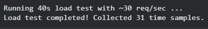
print("Running 40s load test with ~30 req/sec ...")
asyncio.run(run_load())
metrics = loop.run_until_complete(run_load())
print("Load test completed! Collected", len(metrics), "time samples.")
Output:
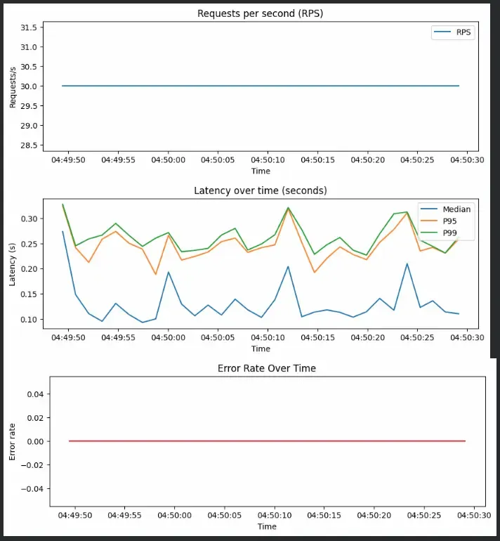
Step 3: Visualizing System Metrics
Once the load test is done, we visualize metrics for RPS, latency and error rate
- RPS Chart: Reflects throughput stability over time.
- Latency Chart: Shows model responsiveness under mixed workloads.
- Error Chart: Detects request failures during overload conditions.
times = [datetime.fromtimestamp(m["time"]) for m in metrics]
rps = [m["rps"] for m in metrics]
p95 = [m["p95"] for m in metrics]
p99 = [m["p99"] for m in metrics]
median = [m["median"] for m in metrics]
error_rate = [m["error_rate"] for m in metrics]

plt.figure(figsize=(10, 3))
plt.plot(times, rps, label="RPS")
plt.title("Requests per second (RPS)")
plt.xlabel("Time")
plt.ylabel("Requests/s")
plt.legend()
plt.show()

plt.figure(figsize=(10, 3))
plt.plot(times, median, label="Median")
plt.plot(times, p95, label="P95")
plt.plot(times, p99, label="P99")
plt.title("Latency over time (seconds)")
plt.xlabel("Time")
plt.ylabel("Latency (s)")
plt.legend()
plt.show()

plt.figure(figsize=(10, 3))
plt.plot(times, error_rate, color='red')
plt.title("Error Rate Over Time")
plt.xlabel("Time")
plt.ylabel("Error rate")
plt.show()
Output:
Step 4: Simulating Dynamic Autoscaling
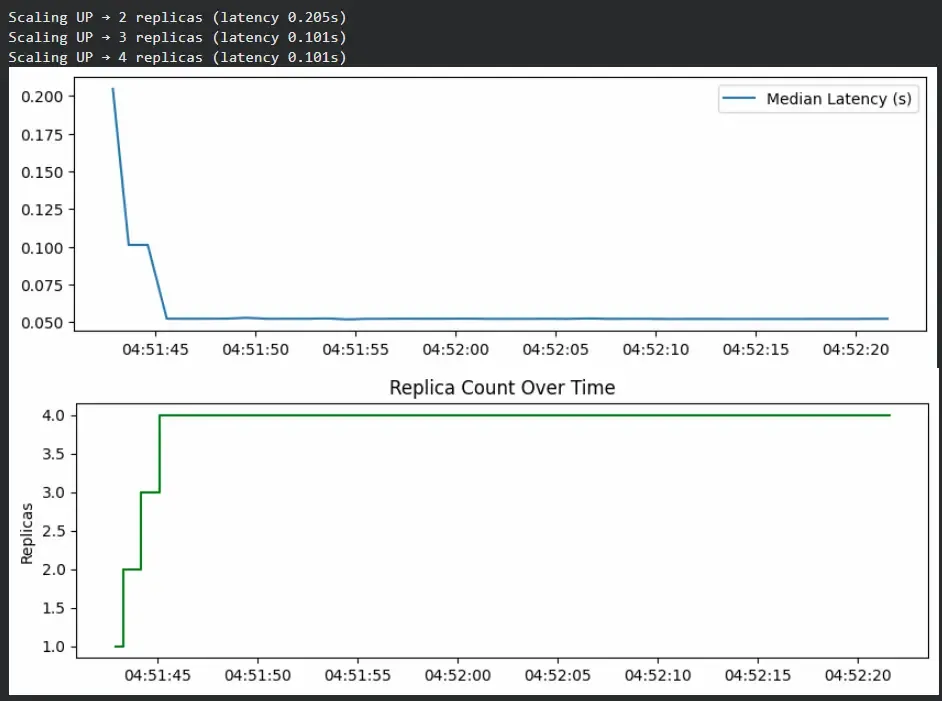
To demonstrate scaling behavior, we simulate a system that automatically increases or decreases replicas based on latency.
- The simulation starts with 1 replica.
- If latency crosses 0.1s, it scales up by adding a replica.
- If latency drops below 0.05s, it scales down to save resources.
- The charts visualize how replicas increase during high latency and stabilize as load decreases.
import concurrent.futures
import numpy as np
import time
from datetime import datetime
import matplotlib.pyplot as plt

replicas = 1
max_replicas = 5
scale_threshold_latency = 0.1


def model_predict(X, work=50):
    time.sleep(work / 1000.0)
    return np.random.choice([0, 1])


def simulate_load_dynamic(duration_s=40, base_rps=30):
    global replicas
    metrics = []
    X_sample = np.random.randn(20)

    for sec in range(duration_s):
        start = time.time()
        rps = base_rps
        lats = []

        with concurrent.futures.ThreadPoolExecutor(max_workers=replicas * 4) as ex:
            futures = [ex.submit(model_predict, X_sample) for _ in range(rps)]
            for f in concurrent.futures.as_completed(futures):
                lats.append(time.time() - start)

        median_lat = np.median(lats)
        metrics.append({
            "time": datetime.now(),
            "replicas": replicas,
            "median": median_lat
        })

        if median_lat > scale_threshold_latency and replicas < max_replicas:
            replicas += 1
            print(
                f"Scaling UP → {replicas} replicas (latency {median_lat:.3f}s)")
        elif median_lat < 0.05 and replicas > 1:
            replicas -= 1
            print(f"Scaling DOWN → {replicas} replicas")

        delay = 1 - (time.time() - start)
        if delay > 0:
            time.sleep(delay)

    return metrics


metrics = simulate_load_dynamic()
times = [m["time"] for m in metrics]
plt.figure(figsize=(10, 3))
plt.plot(times, [m["median"] for m in metrics], label="Median Latency (s)")
plt.legend()
plt.show()

plt.figure(figsize=(10, 3))
plt.step(times, [m["replicas"] for m in metrics], where='mid', color='green')
plt.title("Replica Count Over Time")
plt.ylabel("Replicas")
plt.show()
Output:
Real-World Monitoring and Scaling Tools
Let's see some tools that are often used to handle monitoring and scaling.
| Tool | Purpose | Description |
|---|---|---|
| Prometheus | Monitoring | Collects and stores real-time metrics such as latency, RPS and CPU usage. |
| Grafana | Visualization | Builds dashboards to visualize metrics and alert on anomalies. |
| Kubernetes HPA (Horizontal Pod Autoscaler) | Autoscaling | Dynamically adjusts the number of model pods based on CPU, GPU or custom metrics. |
| Ray Serve / BentoML | Model Serving | Manages scalable deployment and load balancing for ML models. |
| ELK Stack (Elasticsearch, Logstash, Kibana) | Logging | Aggregates and visualizes logs for troubleshooting and trend analysis. |
Advantages
- Maintains model responsiveness under heavy load.
- Enables cost-efficient infrastructure usage.
- Detects performance drift or anomalies early.
- Prevents downtime through proactive scaling.
Limitations
- Autoscaling adds system complexity.
- Monitoring overhead can increase latency slightly.
- Requires careful threshold tuning to avoid oscillations.
- Real-world scaling may depend on deployment platform constraints like Kubernetes, Ray Serve, etc.
