RAG System with LangChain and LangGraph

In this article we will build a Retrieval-Augmented Generation (RAG) system that improves AI answers by combining large language models with a smart document search. It reads documents, breaks them into smaller parts, turns them into searchable vectors. When user queries it uses context from documents to produce accurate, context-aware answers. Here we will also use:

• LangChain which loads and splits documents into chunks, creates vector embeddings to represent text and interfaces with language models to generate answers.
• LangGraph controls the order of retrieval and generation steps, manages state and data flow across the system and enables modular, maintainable AI workflows.

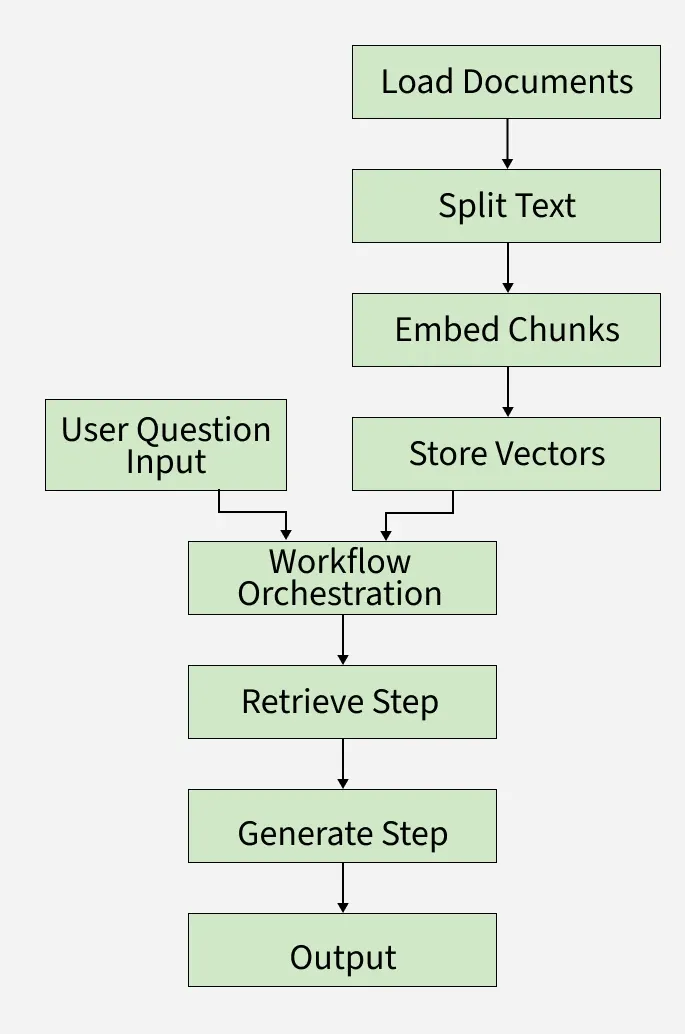
As we can see in the workflow,

• Documents are loaded and read using LangChain.
• Documents are split into smaller text chunks.
• Each chunk is converted into a vector embedding for fast searching.
• When a user asks a question, it is sent to the LangGraph workflow.
• LangGraph orchestrates the process, using stored vectors and the user query.
• The system retrieves relevant chunks using LangChain’s search.
• LangChain and LangGraph together generate a smart answer using a language model.
• The final answer is presented back to the user.

Step-by-Step Implementation

Let's build a RAG system with the help of LangChain and LangGraph:

Step 1: Install Dependencies

We will install the require packages that will be needed such as langchain, langgraph, langchain-openai, langchain-text-splitter, langchain-community, networkx and matplotlib.

!pip install langchain langgraph langchain-openai langchain-text-splitters langchain-community networkx matplotlib

Step 2: Setup API Keys

We configure the environment variable for the OpenAI API key. This is required to authenticate and access OpenAI models.

• os.environ["OPENAI_API_KEY"]: Sets the API key as an environment variable so that LangChain/OpenAI libraries can automatically pick it up when calling the model.

To know how to acess

import os

os.environ["OPENAI_API_KEY"] = "openai_API_key"

Step 3: Define the Application State

We define a TypedDict called State to represent the flow of data across our RAG pipeline.

• question: The user’s query.
• context: A list of retrieved Document objects relevant to the query.
• answer: The final generated response from the language model.

from typing_extensions import TypedDict, List
from langchain_core.documents import Document


class State(TypedDict):
    question: str
    context: List[Document]
    answer: str

Step 4: Load and Split Documents

Used knowledge based file can be downloaded from here.

We will unzip, loads documents and split it into smaller chunks.

• RecursiveCharacterTextSplitter: Breaks down long documents into chunks (chunk_size=1000) with overlap (chunk_overlap=200) to maintain context.

import json
from langchain_core.documents import Document

with open('knowledge_base.json', 'r') as f:
    knowledge_items = json.load(f)

local_docs = [Document(page_content=item['text']) for item in knowledge_items]

Step 5: Create Embeddings and Vector Store

We convert the document chunks into embeddings and store them in a vector database for similarity search.

• OpenAIEmbeddings: Generates embeddings using OpenAI’s embedding model text-embedding-3-large.
• InMemoryVectorStore: A lightweight in-memory store for embeddings.
• add_documents: Stores the vector representations of all document chunks.

from langchain.embeddings import OpenAIEmbeddings
from langchain_core.vectorstores import InMemoryVectorStore
from langchain.text_splitter import RecursiveCharacterTextSplitter

text_splitter = RecursiveCharacterTextSplitter(chunk_size=1000, chunk_overlap=200)
all_splits = text_splitter.split_documents(local_docs)


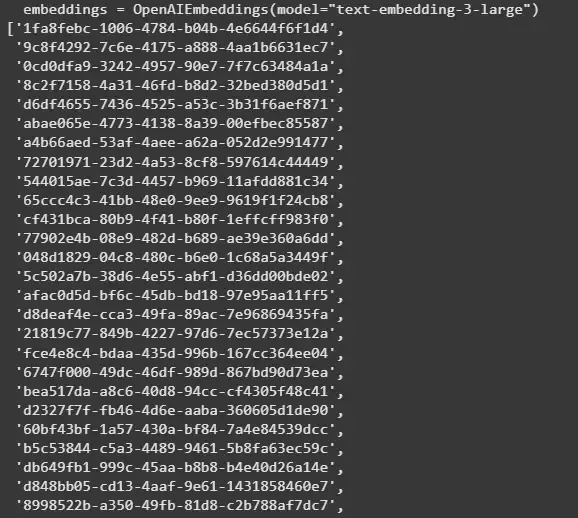
embeddings = OpenAIEmbeddings(model="text-embedding-3-large")
vector_store = InMemoryVectorStore(embeddings)
vector_store.add_documents(all_splits)

Output:

Step 6: Define Custom Prompt and Initialize LLM Model

Define a custom prompt template guiding the LLM to use retrieved context to answer user questions clearly and concisely. Initialize OpenAI GPT-4.1 chat model with temperature 0.3 for manageable creativity in answers.

from langchain.chat_models import init_chat_model
CUSTOM_PROMPT = """
You are an advanced assistant. Use the context to answer. If insufficient info, say so clearly.

Question: {question}

Context:
{context}

Answer:
"""

llm = init_chat_model("openai:gpt-4.1", temperature=0.3)

Step 7: Define Workflow Functions

Define individual LangGraph node functions for each pipeline step:

• retrieve(state): Perform similarity search on the vector store to get top 5 matched document chunks related to the question.
• generate(state): Format the prompt with question + retrieved context, invoke the LLM and return the generated answer.
• classify(state): Dummy function that identifies "advanced" questions but currently passes the question unchanged.
• refine(state): Append a refinement note to the generated answer for clarity.

def retrieve(state: State):
    retrieved_docs = vector_store.similarity_search(state["question"], k=5)
    return {"context": retrieved_docs}


def generate(state: State):
    docs_content = "\n\n".join(doc.page_content for doc in state["context"])
    prompt_filled = CUSTOM_PROMPT.format(
        question=state["question"], context=docs_content)
    response = llm.invoke([{"role": "user", "content": prompt_filled}])
    return {"answer": response.content}


def classify(state: State):
    is_advanced = "advanced" in state["question"].lower()
    return {"question": state["question"]}


def refine(state: State):
    refined_answer = state["answer"] + \
        "\n\n[Refined for clarity and completeness]"
    return {"answer": refined_answer}

Step 8: Build the LangGraph Workflow

We define the pipeline as a graph using LangGraph.

• StateGraph(State): Defines a graph where nodes pass along State.
• add_sequence([retrieve, generate]): Runs retrieval first, then generation.
• add_edge(START, "retrieve"): Connects the start of the graph to the first node.
• compile(): Finalizes the graph for execution.

from langgraph.graph import START, StateGraph

graph_builder = StateGraph(State).add_sequence(
    [classify, retrieve, generate, refine])
graph_builder.add_edge(START, "classify")
graph = graph_builder.compile()

Step 9: Visualize the LangGraph Workflow

Using NetworkX and Matplotlib, we will visualize our workflow,

• G = nx.DiGraph(): Creates an empty directed graph where edges have direction, modeling workflow steps.
• nx.draw_networkx_nodes(...): Draws graph nodes with specified colors, sizes and borders.
• nx.draw_networkx_edges(...): Draws arrows between nodes with custom style and curvature for clarity.
• plt.title(), plt.tight_layout(), plt.axis('off'): Sets title, adjusts layout and hides axes for a clean plot.

import networkx as nx
import matplotlib.pyplot as plt


def visualize_langgraph_clean(graph_builder):
    G = nx.DiGraph()
    for node_name in graph_builder.nodes:
        G.add_node(node_name)
    for src, tgt in graph_builder.edges:
        G.add_edge(src, tgt)

    try:
        pos = nx.nx_agraph.graphviz_layout(G, prog='dot')
    except Exception:
        pos = nx.spring_layout(G, seed=42, k=1.2)

    node_styles = {
        "__start__": {"color": "#666666", "size": 3500},
        "classify": {"color": "#56c2ff", "size": 3300},
        "retrieve": {"color": "#75ff90", "size": 3300},
        "generate": {"color": "#ff8888", "size": 3300},
        "refine": {"color": "#b996fa", "size": 3500}
    }
    node_colors = [node_styles.get(node, {"color": "#cccccc"})[
        "color"] for node in G.nodes()]
    node_sizes = [node_styles.get(node, {"size": 2700})[
        "size"] for node in G.nodes()]

    nx.draw_networkx_nodes(G, pos, node_color=node_colors,
                           node_size=node_sizes, edgecolors='#303030', alpha=0.93)
    nx.draw_networkx_edges(G, pos, arrows=True, arrowstyle='-', arrowsize=25,
                           width=3, edge_color='#555', alpha=0.75, connectionstyle='arc3,rad=0.08')
    nx.draw_networkx_labels(G, pos, font_size=17,
                            font_weight='bold', font_family='sans-serif')

    plt.title("LangGraph Workflow", fontsize=18, fontweight='bold', pad=15)
    plt.tight_layout()
    plt.axis('off')
    plt.show()


visualize_langgraph_clean(graph_builder)

Output:

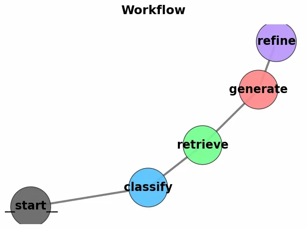
With the help of langgraph we were able to visualize workflow of our application which is helpful for better communication and understanding.

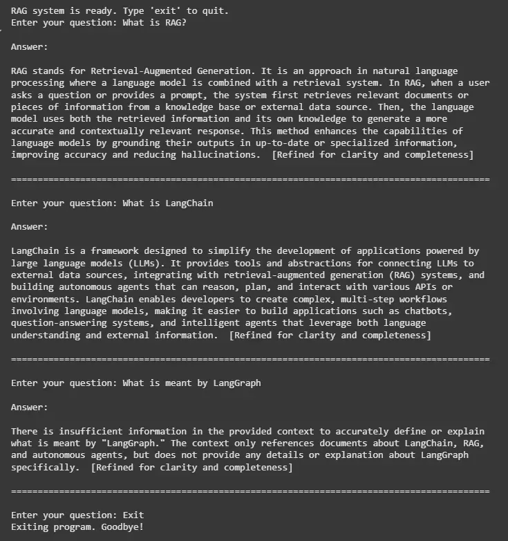
Step 10: Run the System

We take user input, pass it through the graph and display the answer.

• graph.invoke(): Executes the graph pipeline (retrieve: generate).

print("RAG system is ready. Type 'exit' to quit.")

while True:
    question = input("Enter your question: ")
    if question.lower() in ("exit", "quit", "stop"):
        print("Exiting program. Goodbye!")
        break

    response = graph.invoke({"question": question})
    answer = response.get("answer", "No answer generated.")
    print("\nAnswer:\n")
    print(answer)
    print("\n" + "=" * 90 + "\n")

Output:

Advantages

Let's see the advantages that are offered by this system:

• Grounded Responses: Unlike vanilla LLMs that may hallucinate, RAG grounds the model’s answers in actual documents, improving factual accuracy.
• Domain Adaptability: We can easily load custom datasets (PDFs, web pages, internal notes) and make the system specialized for finance, healthcare, legal, research, etc.
• Up-to-date Knowledge: The system retrieves the latest information from external sources, overcoming the LLM’s fixed training cutoff.
• Efficient Context Management: By using document chunking and vector search, the model only processes the most relevant text instead of the entire dataset, reducing token costs and speeding up inference.