Spectral analysis is a powerful technique used to explore the frequency components of time series data. Rather than analyzing variations over time, it shifts the focus to the frequency domain, examining how the signal's energy or variance is distributed across different frequencies. This approach is especially valuable for uncovering hidden periodicities, cyclic behavior, and structural patterns that might remain obscured in the time domain representation.
Spectral Analysis
Spectral Analysis is a way to study time series data by looking at its frequencies instead of how it changes over time. It breaks down complex signals into basic waves to help find repeating patterns, cycles, or hidden details that might be hard to see in regular time-based analysis.
Spectral analysis methods
- Fourier Transform (FT): Breaks down a time series into a combination of sine and cosine waves to show what frequencies are present.
- Fast Fourier Transform (FFT): A faster version of the Fourier Transform that is widely used in practice.
- Periodogram: A plot that shows how much signal energy is present at each frequency. It helps visualize repeating patterns.
- Welch’s Method: Improves the periodogram by splitting the data into overlapping parts, averaging them to reduce noise.
- Lomb-Scargle Periodogram: A version of the periodogram that works well even when the data is unevenly spaced or has gaps.
- Wavelet Transform: Breaks down the time series into both time and frequency components. Good for signals that change over time.
- Short-Time Fourier Transform (STFT): Like the Fourier Transform, but applied in small time windows, so it shows how frequencies change over time.
Why Use Spectral Analysis?
Time series data can often appear noisy or random in the time domain, especially when multiple components with different frequencies are mixed together. Spectral analysis helps:
- Identify dominant cycles or periodic behavior.
- Remove noise by filtering certain frequencies.
- Diagnose system behavior in control and signal systems
Time-Domain vs. Frequency-Domain Analysis
- Time-Domain Analysis: Observes variations in a signal over time.
- Frequency-Domain Analysis: Examines the contribution of different frequency components to the overall signal.
Spectral analysis shifts data from the time domain to the frequency domain, typically using transformations like the Fourier Transform.
Fourier Transform
The Fourier Transform decomposes a time-domain signal into its individual frequency components.
X(k) = \sum_{n=0}^{N-1} x(n) e^{-j2\pi k n / N}
Fast Fourier Transform (FFT): FFT is an optimized algorithm for computing the DFT efficiently, reducing computational complexity from 𝑂(𝑁2) to 𝑂(𝑁log𝑁).
Power Spectral Density (PSD)
PSD provides insights into the power distribution across different frequency components. It is used to analyze signal strength, periodicities, and spectral characteristics.
PSD is calculated as:
PSD(f) = \frac{1}{N} |X(f)|^2
where ∣𝑋(𝑓)∣2 represents the squared magnitude of the Fourier coefficients.
Periodogram Method
The periodogram estimates the PSD by computing the squared magnitude of the Fourier Transform. It provides insights into the dominant frequencies present in the time series.
Welch’s Method
Welch’s method improves PSD estimation by averaging multiple segments of the signal, reducing noise and improving resolution.
Implementation of Spectral Analysis
import numpy as np
import matplotlib.pyplot as plt
# Sampling rate and time vector
fs = 100 # Samples per second
t = np.linspace(0, 2, 2 * fs, endpoint=False) # 2 seconds of data
# Create a signal with two frequencies
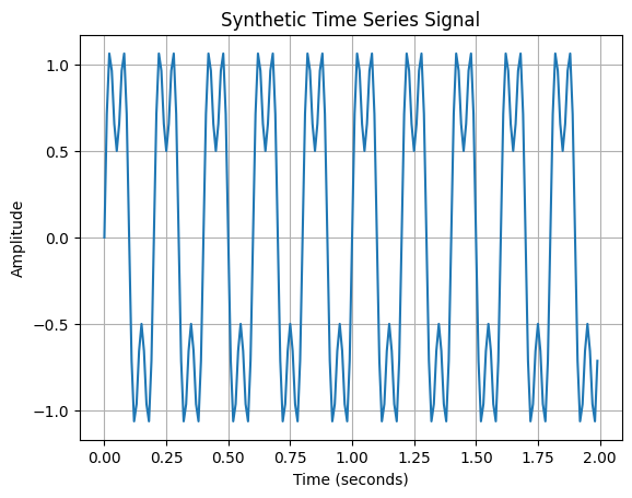
signal = np.sin(2 * np.pi * 5 * t) + 0.5 * np.sin(2 * np.pi * 15 * t)
# Plot the signal
plt.plot(t, signal)
plt.title("Synthetic Time Series Signal")
plt.xlabel("Time (seconds)")
plt.ylabel("Amplitude")
plt.grid(True)
plt.show()
Output
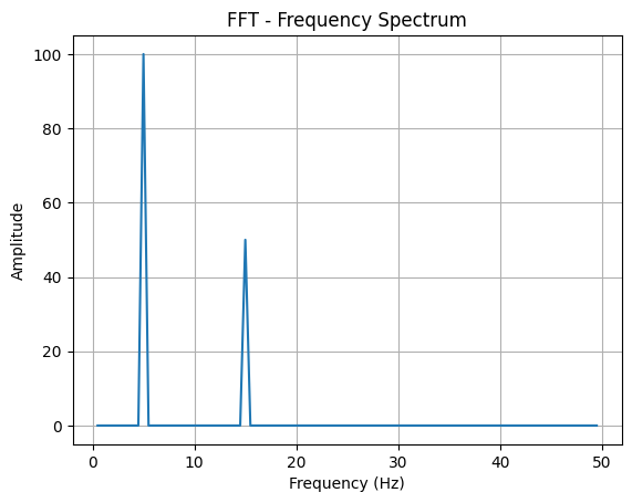
Fast Fourier Transform (FFT)
FFT is the most common and fast way to analyze the frequency content of a time series.
from numpy.fft import fft, fftfreq

# Perform FFT
N = len(t)
fft_values = fft(signal)
fft_freqs = fftfreq(N, 1/fs)

# Only keep the positive frequencies
mask = fft_freqs > 0

plt.plot(fft_freqs[mask], np.abs(fft_values[mask]))
plt.title("FFT - Frequency Spectrum")
plt.xlabel("Frequency (Hz)")
plt.ylabel("Amplitude")
plt.grid(True)
plt.show()
Output
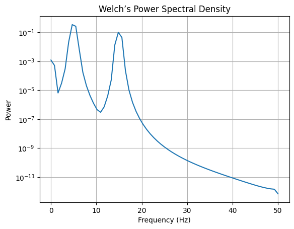
Power Spectral Density (PSD) using Welch's Method
Welch’s method is a cleaner way to estimate the power at each frequency by averaging over segments of the data.
from scipy.signal import welch

frequencies, psd = welch(signal, fs, nperseg=128)

plt.semilogy(frequencies, psd)
plt.title("Welch’s Power Spectral Density")
plt.xlabel("Frequency (Hz)")
plt.ylabel("Power")
plt.grid(True)
plt.show()
Output
Applications of Spectral Analysis
- Signal Processing- Used in audio, image processing, and speech recognition to analyze and filter signals.
- Financial Market Analysis- Helps detect cycles in stock prices and economic indicators.
- Biomedical Engineering- Spectral methods analyze heart rate variability and EEG brain signals.
- Climate Science- Examines seasonal trends and long-term climate changes.
- Speech and Audio Analysis- Used in speech recognition systems to distinguish different frequency components.
