A feedback system in neural networks is a mechanism where the output is fed back into the network to influence subsequent outputs, often used to enhance learning and stability.
This article provides an overview of the working of the feedback loop in Neural Networks.
Understanding Feedback System
In dynamic systems, feedback is a crucial mechanism where the output from a component cycles back to influence the input to that same component. This interaction forms closed-loop pathways that allow the system to self-regulate and adjust based on performance. Such feedback loops can be positive or negative, amplifying or diminishing the system's response, respectively. In the context of neural networks, feedback mechanisms are essential for creating more accurate models. Traditional feedforward neural networks process information in one direction, from input to output, without any looping back.
Types of Neural Networks with Feedback Systems
Neural networks with feedback systems, like RNNs, use their internal state to process sequences of inputs. Here are three main types:
1. Recurrent Neural Networks (RNNs):
Recurrent Neural Networks (RNNs) recognize patterns in sequences of data like time series or text. They use a hidden state to process variable-length sequences.
Key Features:
- Feedback Loop: Maintains a hidden state.
- Sequential Processing: Good for tasks needing context, like language modeling.
2. Long Short-Term Memory (LSTM) Networks:
Long Short-Term Memory (LSTM) Networks handle long-term dependencies and solve the vanishing gradient problem. They have gates to control information flow.
Key Features:
- Forget Gate: Discards information from cell state.
- Input Gate: Stores new info in cell state.
- Output Gate: Decides what to output.
3. Gated Recurrent Unit (GRU) Networks:
Gated Recurrent Unit (GRU) Networks are simpler than LSTMs, combining forget and input gates into an update gate.
Key Features:
- Update Gate: Controls info flow to the hidden state.
- Reset Gate: Decides how much past info to forget.
Mechanisms of Feedback in Neural Network
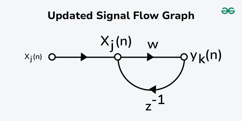
Here is a signal flow graph of a neural network that considers feedback.

Where,
- xj(n) is the input signal.
- x`j(n) is the internal signal.
- yk(n) is the output signal.
- A is feedforward transmission.
- B is feedback transmission.
Equations associated with the graph
These signals are functions of the discrete – time variable (n). The system is assumed to be linear, consisting of forward path and feedback path that are characterized by the operators A and B respectively.
from eq. (1) and (2) , we can rewrite yk(n) as:
where,
- A/(1-AB) is the closed loop operator of the system.
- AB is the open loop operator and BA ≠ AB.
Now Suppose A as fixed weight "W", B as a unit delay operator z-1 , whose output is delayed with respect to the input by “one time unit”. We may then express the closed loop operator of the system as:
Using binomial expansion for (1 – w-1) -1 , we may rewrite the closed loop operator of the system as:
Substituting this eq. into eq. (3)
From the definition of z-1 , we have
where xj(n-l) is a sample of the input signal delayed by l time units.
Accordingly, we may express the output signal yk(n) as an infinite weighted summation of present and past samples of the input signal xj(n), as shown by:
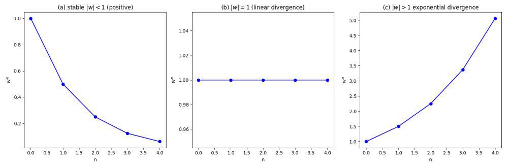
We now see clearly that the dynamic behavior of a feedback system represented by the signal-flow graph is controlled by the weight w.
In particular two specific cases can be distinguished:
- |w| < 1, the output signal yk(n) is exponentially convergent, that is the system is stable.
- |w| > 1, the output signal yk(n) is divergent, that is, the system is unstable.
- If |w| = 1 the divergence is linear, and if |w| >1 the divergence is exponential.
Simulation of Feedback System Dynamics for Various Feedback Parameters
This code represents the simulation of a feedback system, demonstrating how different values of the feedback parameter w affect the stability and behavior of the system's output over time.
feedback_system(xj, w, num_samples): This function computes the output of the feedback system given an input signalx_j , a feedback parameterw, and the number of samplesnum_samples.x_j is the input signal, which is a step function in this case (all ones).y_k is initialized as a zero array to store the output signal.- The nested loops compute the output
ykbased on the feedback system's equation:y_k(n) = \sum_{l=0}^{n} (w^{l+1}) x_j(n-l) . This equation indicates that the output at timenis a weighted sum of past inputs, with the weights being powers ofw.
# Ensure you have the necessary libraries installed:
# You can uncomment the following lines to install the required packages if not already installed.
# !pip install numpy matplotlib

import numpy as np
import matplotlib.pyplot as plt

def feedback_system(xj, w, num_samples):
    yk = np.zeros(num_samples)
    for n in range(num_samples):
        for l in range(n + 1):
            yk[n] += (w ** (l + 1)) * xj[n - l]
    return yk

# Parameters
num_samples = 50
xj = np.ones(num_samples)  # Input signal: a step function
weights = [0.5, 1.0, 1.2]  # Different values of w to demonstrate stability and instability

# Plotting the results
plt.figure(figsize=(12, 8))

for w in weights:
    yk = feedback_system(xj, w, num_samples)
    plt.plot(yk, label=f'w = {w}')

plt.title('Output of Feedback System for Different Weights')
plt.xlabel('Time (n)')
plt.ylabel('Output Signal y_k(n)')
plt.legend()
plt.grid(True)
plt.show()
Output:
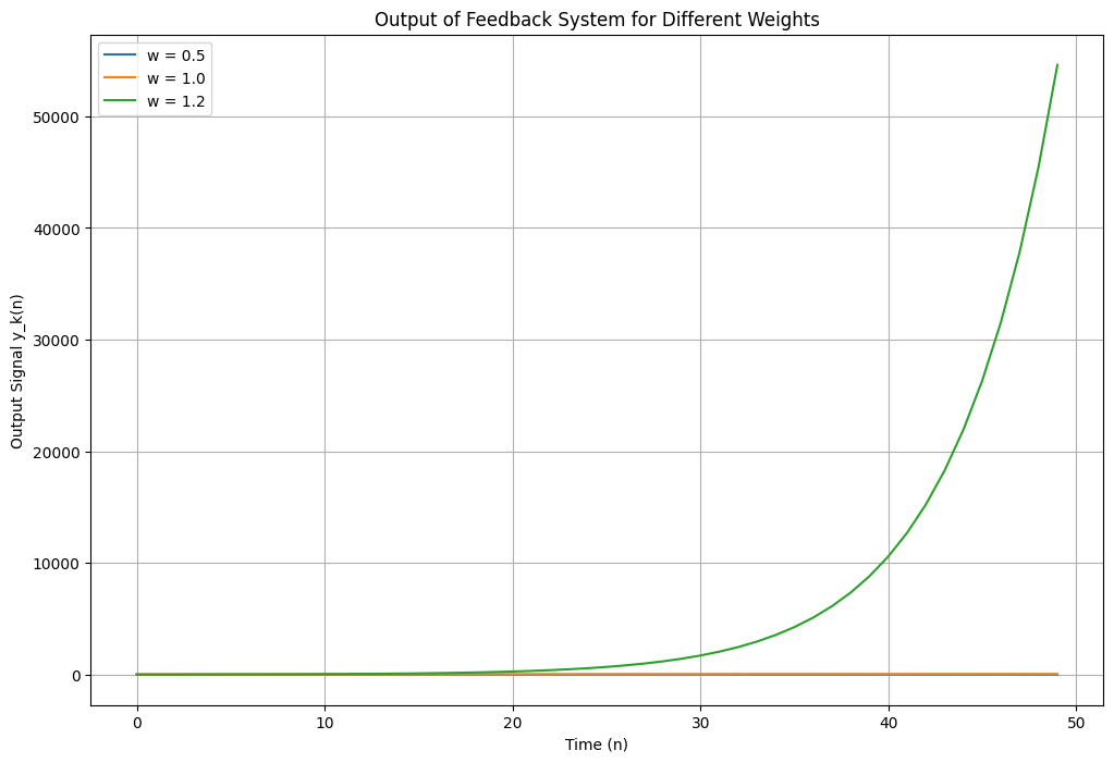
Explanation of the System's Behavior
- Stable System (
|w| < 1): When ∣w∣|w|∣w∣ is less than 1 (e.g., w=0.5w = 0.5w=0.5), the output signal stabilizes because the feedback effect diminishes over time. - Marginally Stable System (
|w| = 1): When ∣w∣|w|∣w∣ is equal to 1 (e.g., w=1.0w = 1.0w=1.0), the output signal shows linear growth or constant behavior, indicating marginal stability. - Unstable System (
|w| > 1): When ∣w∣|w|∣w∣ is greater than 1 (e.g., w=1.2w = 1.2w=1.2), the output signal grows exponentially, indicating an unstable system due to the increasing effect of feedback over time.
Advantages of Feedback Mechanisms
- Stability: Helps maintain system stability by self-regulating.
- Accuracy: Improves accuracy by continuously adjusting based on output.
- Adaptability: Allows systems to adapt to changing conditions and inputs.
- Error Correction: Identifies and corrects errors in real-time.
- Efficiency: Enhances system efficiency by optimizing performance.
- Robustness: Increases robustness against disturbances and uncertainties.
Conclusion
Feedback mechanisms in dynamic systems play a vital role in self-regulation and adjustment based on system performance. This principle is fundamental in neural networks, where feedback can create more accurate models compared to traditional feedforward neural networks. By incorporating feedback, systems can use past outputs to influence current inputs, forming a closed-loop pathway that affects system stability and performance.
