Perceptron Convergence Theorem in Neural Networks

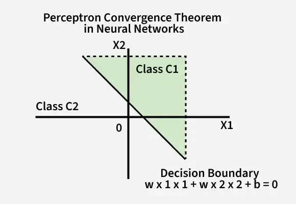
The Perceptron Convergence Theorem explains when a perceptron can successfully learn a classification task. It states that if the training data is linearly separable, the perceptron algorithm will eventually find a decision boundary that correctly classifies all training examples.

• Guarantees convergence for linearly separable data
• Forms the foundation of perceptron learning
• Helps understand classification and decision boundaries

Statement of Perceptron Convergence Theorem

The Perceptron Convergence Theorem states that if a set of training examples is linearly separable, then the perceptron learning algorithm is guaranteed to converge to a weight vector that correctly classifies all training examples after a finite number of updates.

Conditions for Convergence

For the perceptron algorithm to converge, the following conditions must be satisfied:

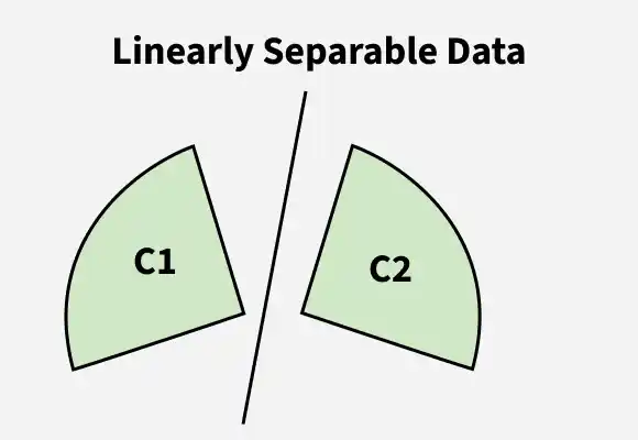
• Linear Separability: The data must be separable by a linear boundary (hyperplane).
• Non-Zero Margin: A positive margin must exist between the classes.

The convergence condition can be expressed as:

y_i (w⋅x_i +b)≥γ

Where w is the weight vector, b is the bias, and γ is the margin.

Implications for Theorem

• Convergence: The perceptron is guaranteed to find a decision boundary for linearly separable data.
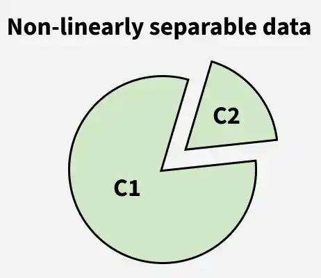
• Non-Convergence: If the data is not linearly separable, the perceptron will continue updating its weights and may never converge.

1. Linearly Separable Data: Classes can be separated using a straight line, plane, or hyperplane.

2. Non-Linearly Separable Data: No single linear boundary can perfectly separate the classes.

Mathematical Formulation

To simplify the notation, the bias is treated as an additional weight associated with a fixed input value of +1.

• Input vector : x(n) = [+1, x_1(n), x_2(n), \ldots, x_m(n)] where n is the iteration step of the algorithm.
• Weight vector : w(n) = [b(n), w_1(n), w_2(n), \ldots, w_m(n)]
• Linear combiner output : v(n) = \Sigma_{i=1}^m w_i(n)x_i(n) = w^T(n)x(n)

The decision boundary is defined by w^Tx = 0 which represents a hyperplane separating the two classes.

Weight update rule

If a sample is correctly classified, no update is made: w(n+1) = w(n)

Otherwise, the weights are adjusted:

• if w^T(n)x(n)>0 and x(n)\epsilon C2.w(n+1) =w(n)+ \eta x(n),
• if w^T(n)x(n)\leq 0 and x(n)\epsilon C1.

Working

The perceptron learns by iteratively updating its weights based on prediction errors until it finds a decision boundary that correctly classifies the training data.

Step 1: Initialize Parameters

Initialize the weights, bias, learning rate, and number of training epochs.

Step 2: Compute Weighted Sum

Calculate the weighted sum of inputs and bias.

z = w^T x + b

Step 3: Apply Activation Function

Pass the weighted sum through a step function to generate the predicted output.

Step 4: Update Weights

If the prediction is incorrect, update the weights and bias to reduce the classification error.

w_i = w_i + \Delta w_i

b = b +\Delta b

Where:

• \Delta w_i = \eta * (y-y')*x_i
• \Delta b = \eta *(y-y')
• \eta is learning rate parameter
• y is the actual label
• y^{\prime} is the predicted label

Step 5: Repeat Until Convergence

Repeat the process for all training samples until the perceptron correctly classifies the data or the maximum number of epochs is reached.

Implementation

Step 1: Import Libraries

Import the required libraries for numerical computation, visualization, and dataset loading.

import numpy as np
from sklearn.datasets import load_iris
import matplotlib.pyplot as plt

Step 2: Load and Prepare the Dataset

Load the Iris dataset, select the first 100 samples and two features, and convert the target labels into binary classes (-1 and 1).

iris = load_iris()

X = iris.data[:100, :2]

y = iris.target[:100]
y = np.where(y == 0, -1, 1)

Step 3: Initialize Hyperparameters

Initialize the weights, bias, learning rate, and number of training epochs.

weights = np.zeros(X.shape[1])
bias = 0

learning_rate = 0.01
n_iter = 500

Step 4: Define the Perceptron Training Function

• Create a function to train the perceptron model using the learning rule.
• This function computes predictions and updates the weights and bias whenever a sample is misclassified.

def train_perceptron(X, y, weights, bias, learning_rate, n_iter):
    for epoch in range(n_iter):
        for idx, x_i in enumerate(X):

            linear_output = np.dot(x_i, weights) + bias

            y_predicted = np.where(linear_output >= 0, 1, -1)

            update = learning_rate * (y[idx] - y_predicted)

            weights += update * x_i
            bias += update

    return weights, bias

Step 5: Train the Perceptron

• Train the perceptron using the prepared dataset.
• After training, the model returns the optimized weights and bias.

weights, bias = train_perceptron(
    X,
    y,
    weights,
    bias,
    learning_rate,
    n_iter
)

Step 6: Define the Prediction Function

Create a function to predict class labels using the trained model.

def predict(X, weights, bias):
    linear_output = np.dot(X, weights) + bias
    return np.where(linear_output >= 0, 1, -1)

Step 7: Generate Predictions

Use the trained perceptron to classify the samples.

y_pred = predict(X, weights, bias)

Step 8: Evaluate Model Accuracy

Calculate the prediction accuracy of the trained model.

accuracy = np.mean(y_pred == y)

print(f"Accuracy: {accuracy * 100:.2f}%")

Output:

Accuracy: 99.00%

Step 9: Create a Function to Plot the Decision Boundary

Define a function to visualize the decision boundary learned by the perceptron.

def plot_decision_boundary(X, y, weights, bias):
    x_min, x_max = X[:, 0].min() - 1, X[:, 0].max() + 1
    y_min, y_max = X[:, 1].min() - 1, X[:, 1].max() + 1

    xx, yy = np.meshgrid(
        np.arange(x_min, x_max, 0.01),
        np.arange(y_min, y_max, 0.01)
    )

    Z = predict(
        np.c_[xx.ravel(), yy.ravel()],
        weights,
        bias
    )

    Z = Z.reshape(xx.shape)

    plt.contourf(xx, yy, Z, alpha=0.3)
    plt.scatter(
        X[:, 0],
        X[:, 1],
        c=y,
        marker='o',
        edgecolor='k'
    )

    plt.show()

Step 10: Visualize the Decision Boundary

Plot the decision boundary generated by the perceptron.

plot_decision_boundary(X, y, weights, bias)

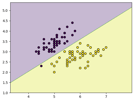
The resulting plot shows the decision boundary learned by the perceptron, illustrating how the model separates the two classes based on the selected features.

You can download the source code from here.

Advantages

• Simple and easy to implement for binary classification problems.
• Guarantees convergence when the training data is linearly separable.
• Learns efficiently and often converges quickly on well-separated datasets.
• Provides a strong theoretical foundation for understanding neural network learning.

Limitations

• Works only when the data is linearly separable.
• Performance can be affected by noisy or overlapping data.
• Cannot directly handle multi-class classification tasks.
• May fail to learn complex non-linear decision boundaries.