PyTorch-Lightning Conda Setup Guide

PyTorch-Lightning is a popular deep learning framework and is more simple version of PyTorch. It is easy to use as one does not need to define the training loops and the testing loops. We can perform distributed training easily without making the code complex. Some other features include more focus on research rather than code, easy debugging etc.

Installing Conda for PyTorch Lightning

Conda is an open source software that provides support of various languages like R, Python,Java and Ruby. It is free to use. Also users can create isolated environments and download the required packages. There are two main versions of conda: Anaconda and Miniconda. To install conda follow these steps:

• Download the Anaconda or Miniconda installer from official website.
• Double click on .exe file.
• Agree to Terms and conditions and also select whether to install for that particular user or for all users.
• Browse and select the location where conda should be installed.
• Ensure that the Conda has been added to the path variable.

Creating and Activating Conda Environment

To create and activate Conda Environment we can use Command Prompt or Anaconda Prompt. For users using Command prompt, ensure that Conda is added to the path variables. The steps are as follows:

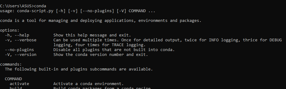
1. Open Command prompt and type conda:

2. Use the Create Command to Create an Environment.

conda create --name myproject python=3.10

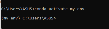
3. Activate the Environment:

conda activate myprojectname

Installing PyTorch-Lightning Using Conda

To install PyTorch-Lightning we have to first install PyTorch. Now we can install PyTorch for CPU as well as GPU. The commands are as follows:

For CPU

conda install pytorch torchvision torchaudio cpuonly -c pytorch

For GPU with CUDA

conda install pytorch torchvision torchaudio pytorch-cuda=11.7 -c pytorch -c nvidia

To install PyTorch Lightning use pip command:

pip install pytorch-lightning

Verifying the Installation

To verify that everything is set up correctly, you can open a Python interpreter and try importing both PyTorch and PyTorch Lightning:

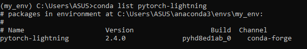
Before building models using PyTorch-Lightning we need to ensure that it has been installed correctly in the virtual environment. To check the installation use conda list command.

Best Practices for Using Conda with PyTorch Lightning

1. Managing Environment YAML Files

Conda allows you to export your environment configuration into a YAML file. This is particularly useful when you want to share your environment setup with others or move it to a different machine.

conda env export > environment.yml

To recreate the environment, the recipient can use:

conda env create -f environment.yml

2. Keeping Packages Updated

Keeping your packages updated ensures that you are working with the latest features and security patches. You can update Conda packages using:

conda update --all

3. Managing Multiple Conda Environments

Conda allows you to manage multiple environments on the same machine. You can list all environments with:

conda env list

To deactivate an environment and return to the base environment, use:

conda deactivate

Example : Creating a Model in PyTorch Lightning Environment with Conda

Here we have used MNIST dataset and created a feed forward neural network. So we will now import the necessary libraries. The dataset is present in the torchvision library.

import pytorch_lightning as pl
import torch
from torch import nn
from torch.utils.data import DataLoader
from torchvision import transforms, datasets

Define Class and the methods

Now we will define the model. The model is defined using class and this class inherits pl.LightningModule. The Lightning Module class takes care of the raining and testing loops.

class LitModel(pl.LightningModule):
    def __init__(self):
        super().__init__()
        self.layer_1 = nn.Linear(28 * 28, 128)
        self.layer_2 = nn.Linear(128, 256)
        self.layer_3 = nn.Linear(256, 10)
        self.loss_fn = nn.CrossEntropyLoss()

Here we have defined three layers and also we have used the Cross Entropy loss to calculate the loss.

After defining the network part of the model, we will now use the forward pass. It basically flattens the input, uses ReLU as Activation function and the final layer is output layer

def forward(self, x):
    x = x.view(x.size(0), -1)
    x = torch.relu(self.layer_1(x))
    x = torch.relu(self.layer_2(x))
    x = self.layer_3(x)
    return x

After defining the forward pass, we will now define the training step of the model. This method basically aims to train the model on each batch, predict, calculate accuracy and loss. The metrics are logged using TensorBoard which can be viewed on the User Interface.

def training_step(self, batch, batch_idx):
    x, y = batch
    y_hat = self(x)
    loss = self.loss_fn(y_hat, y)
    acc = (y_hat.argmax(dim=1) == y).float().mean()
    self.log('train_loss', loss)
    self.log('train_acc', acc)
    return loss

Now to validate the model and stop it from overfitting, we will define the validation_step method.

def validation_step(self, batch, batch_idx):
    x, y = batch
    y_hat = self(x)
    loss = self.loss_fn(y_hat, y)
    acc = (y_hat.argmax(dim=1) == y).float().mean()
    self.log('val_loss', loss, prog_bar=True)
    self.log('val_acc', acc, prog_bar=True)

After validating the model, we will test to check if our model is predicting correctly or not.

def test_step(self, batch, batch_idx):
    x, y = batch
    y_hat = self(x)
    loss = self.loss_fn(y_hat, y)
    acc = (y_hat.argmax(dim=1) == y).float().mean()
    self.log('test_loss', loss, prog_bar=True)
    self.log('test_acc', acc, prog_bar=True)

Now to optimize the performance of the model we will use Adam Optimizer.

def configure_optimizers(self):
    return torch.optim.Adam(self.parameters(), lr=1e-3)

So from the above we can see that we have basically defined the methods in a class that will pass the inputs through the layers, train the model, calculate loss, optimize, validate and also test the predictive power of the model.

Preparing the dataset

Now we will use transforms method to prepare our MNIST dataset. It basically converts it to tensor and normalizes the tensors as well. The batch size is 32.

transform = transforms.Compose([transforms.ToTensor(), transforms.Normalize((0.5,), (0.5,))])
mnist_train = datasets.MNIST(root='.', train=True, download=True, transform=transform)
mnist_test = datasets.MNIST(root='.', train=False, download=True, transform=transform)

train_loader = DataLoader(mnist_train, batch_size=32)
test_loader = DataLoader(mnist_test, batch_size=32)

Training and testing the model

After preparing the dataset, we will create an object and call the Trainer object. This object will take care of training the model. It will fit the data in the model and will train it for 5 epochs. Here we have defined CPU. For GPU we have to specify the accelerator as GPU and also the quantity as well.

model = LitModel()
trainer = pl.Trainer(max_epochs=5, accelerator='cpu')
trainer.fit(model, train_loader, test_loader)
trainer.test(model, test_loader)

The whole code is as follows:

• After executing the code, a folder named lightning_logs will appear.
• It will contain the metrics and the checkpoint file that will contain the weights that has been generated during training phase.

import pytorch_lightning as pl
import torch
from torch import nn
from torch.utils.data import DataLoader
from torchvision import transforms, datasets

# Step 1: Define the LightningModule
class LitModel(pl.LightningModule):
    def __init__(self):
        super().__init__()
        self.layer_1 = nn.Linear(28 * 28, 128)
        self.layer_2 = nn.Linear(128, 256)
        self.layer_3 = nn.Linear(256, 10)
        self.loss_fn = nn.CrossEntropyLoss()

    def forward(self, x):
        # Flatten the input (28x28 images to 784)
        x = x.view(x.size(0), -1)
        x = torch.relu(self.layer_1(x))
        x = torch.relu(self.layer_2(x))
        x = self.layer_3(x)
        return x

    def training_step(self, batch, batch_idx):
        x, y = batch
        y_hat = self(x)
        loss = self.loss_fn(y_hat, y)
        acc = (y_hat.argmax(dim=1) == y).float().mean()  # Accuracy for training
        self.log('train_loss', loss)
        self.log('train_acc', acc)  # Logging training accuracy
        return loss

    def validation_step(self, batch, batch_idx):
        x, y = batch
        y_hat = self(x)
        loss = self.loss_fn(y_hat, y)
        acc = (y_hat.argmax(dim=1) == y).float().mean()  # Validation accuracy
        self.log('val_loss', loss, prog_bar=True)
        self.log('val_acc', acc, prog_bar=True)  # Logging validation accuracy

    def test_step(self, batch, batch_idx):
        x, y = batch
        y_hat = self(x)
        loss = self.loss_fn(y_hat, y)
        acc = (y_hat.argmax(dim=1) == y).float().mean()  # Testing accuracy
        self.log('test_loss', loss, prog_bar=True)
        self.log('test_acc', acc, prog_bar=True)  # Logging test accuracy

    def configure_optimizers(self):
        return torch.optim.Adam(self.parameters(), lr=1e-3)

# Step 2: Prepare Data
transform = transforms.Compose([transforms.ToTensor(), transforms.Normalize((0.5,), (0.5,))])
mnist_train = datasets.MNIST(root='.', train=True, download=True, transform=transform)
mnist_test = datasets.MNIST(root='.', train=False, download=True, transform=transform)

train_loader = DataLoader(mnist_train, batch_size=32)
test_loader = DataLoader(mnist_test, batch_size=32)

# Step 3: Create Trainer and Train Model
model = LitModel()
trainer = pl.Trainer(max_epochs=5, accelerator='cpu')

# Step 4: Train the model
trainer.fit(model, train_loader, test_loader)

# Step 5: Test the model
trainer.test(model, test_loader)

Output:

As we can see that the test accuracy of our model is 96.71%

Conclusion

Using Conda we have created virtual environments and installed the necessary packages as per our requirements. PyTorch-Lightning works efficiently as it reduces code complexity and also makes it more useful as we do not have to manually set up codes for calculation of logs.