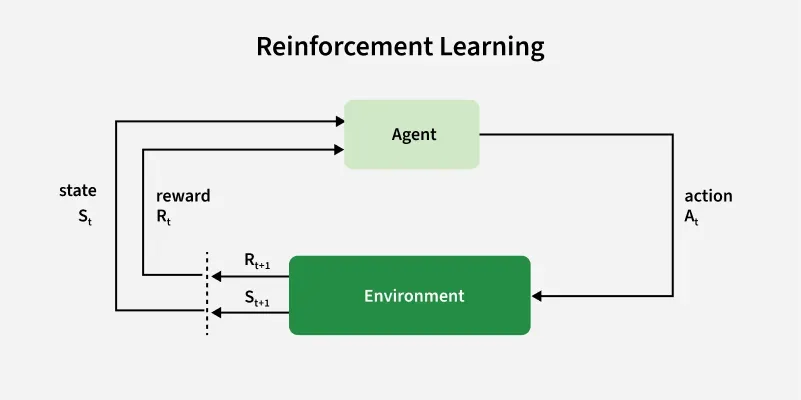
Temporal Difference (TD) learning

Temporal Difference (TD) Learning is a model-free reinforcement learning method used by algorithms like Q-learning to iteratively learn state value functions (V(s)) or state-action value functions (Q(s,a)). Unlike Monte Carlo methods that require full episodes, TD Learning updates value estimates after each time step using the Bellman equation and Temporal Difference error.

How TD Learning Combines Monte Carlo and Dynamic Programming

• Monte Carlo Methods: Learn value estimates by averaging returns after complete episodes. They require the episode to finish before updating values, which makes them unsuitable for continuing (non-episodic) tasks and can lead to high variance in updates.
• Dynamic Programming (DP): Uses a known model of the environment to perform updates by bootstrapping updating value estimates based on other learned values, not just actual returns. DP requires full knowledge of transition and reward probabilities, which is often impractical.

TD Learning: It uses both approaches

• Like Monte Carlo, TD learning does not need a model of the environment (model-free).
• Like DP, TD learning updates predictions based on other learned predictions (bootstrapping), not just actual returns.
• TD methods can learn after every step, not just at episode end, making them suitable for non-episodic and sequential tasks.

Why TD is Model-Free and Non-Episodic

• Model-Free: TD learning does not require knowledge of the environment’s transition or reward structure. It learns directly from experience by updating values based on observed rewards and subsequent predictions.
• Non-Episodic (Sequential): TD learning can update values after every step, not just after an episode ends. This makes it suitable for tasks that do not have clear episode boundaries, such as real-time control or ongoing games.

Core Components

1. Bellman Equation: The foundation for TD updates. For a state value function:

V(s) = \mathbb{E} \left[ R_{t+1} + \gamma V(s_{t+1}) \mid s_t = s \right]

And for Action-Value Function (Q-function)

Q(s, a) = \mathbb{E}_{\pi}\left[ R_{t+1} + \gamma Q(s_{t+1}, a_{t+1}) \mid s_t = s, a_t = a \right]

2. Temporal Difference (TD) Error: \delta_t = R_{t+1} + \gamma V(s_{t+1}) - V(s_t)

3. TD Learning Update Rule: V(s_t) \leftarrow V(s_t) + \alpha \delta_t

4. Expanded TD Update (in one step): The most basic TD algorithm is TD(0), which updates the value function V(s)for state s as follows:

V(s_t) \leftarrow V(s_t) + \alpha \left[ R_{t+1} + \gamma V(s_{t+1}) - V(s_t) \right]

Where:

• V(s_t) : Current estimate for state stst
• R_{t+1} : Reward received after taking action in stst
• γ: Discount factor (how much future rewards are valued)
• V(s_{t+1}) : Estimated value of the next state
• α: Learning rate

The term \left[ R_{t+1} + \gamma V(s_{t+1}) - V(s_t) \right]is called the TD error (\delta_t), representing the difference between the predicted and the newly observed value.

How TD Learning Works: Example with Bellman Equation

Scenario: Assume a grid world with nine squares:

• One "goal" square (+10 reward),
• One "poison" square (–10 reward),
• All other squares (–1 reward per step).

Suppose the agent starts in state S1. The value of each state, V(s), is initialized to zero.

Step 1: Agent Takes an Action

• The agent in S1 randomly chooses to move right to S2.
• It receives a reward R_{t+1} = -1

Step 2: Apply the Bellman Equation

The Bellman equation for the value of a state is:

V(s_t) = \mathbb{E}\left[ R_{t+1} + \gamma V(s_{t+1}) \right]

Suppose \gamma = 0 (for simplicity in this step), and V(S_2) = 0

V_{\text{obs}}(S_1) = R_{t+1} + \gamma V(S_2) = -1 + 0 = -1

Step 3: Calculate Temporal Difference Error

δ t =V obs (S1)−V(S1)=−1−0=−1

Step 4: Update the Value Function

With learning rate \alpha = 0.1

V(S_1) \leftarrow V(S_1) + \alpha \delta_t = 0 + 0.1 \times (-1) = -0.1

Multiple Episodes and Iterative Updates

• Next time step: The agent is now in S2, takes an action (say, moves down to S7), receives a reward (R_{t+1} = -1 ), and the process repeats.
• After each action: The value of the current state is updated using the observed reward and the estimated value of the next state.
• Multiple episodes: This sequence continues for many episodes. Over time, the values in the table converge to reflect the expected total reward from each state under the current policy.
• Policy improvement: Once the value function is learned, the agent can use it to choose actions that maximize expected rewards, shifting from random actions to optimal ones.

This code simulates TD updates for a short sequence. At each step, the value of the current state is updated based on the reward and the value of the next state.

import numpy as np

# Example
states = ['A', 'B', 'C', 'D', 'E']
V = {s: 0.0 for s in states}  # Initialize value function
alpha = 0.1   # Learning rate
gamma = 0.9   # Discount factor

# Simulated experience: (current_state, reward, next_state)
experience = [
    ('B', 0, 'C'),
    ('C', 0, 'D'),
    ('D', 1, 'E'),  # Terminal state E with reward 1
]

for s, r, s_next in experience:
    V[s] = V[s] + alpha * (r + gamma * V[s_next] - V[s])

print(V)

Output

{'A': 0.0, 'B': 0.0, 'C': 0.0, 'D': 0.1, 'E': 0.0}

SARSA and Q-learning are foundational temporal difference (TD) reinforcement learning algorithms that enable agents to learn optimal behaviors through environment interactions. Both use TD error to update action-value estimates but differ fundamentally in policy evaluation approaches.

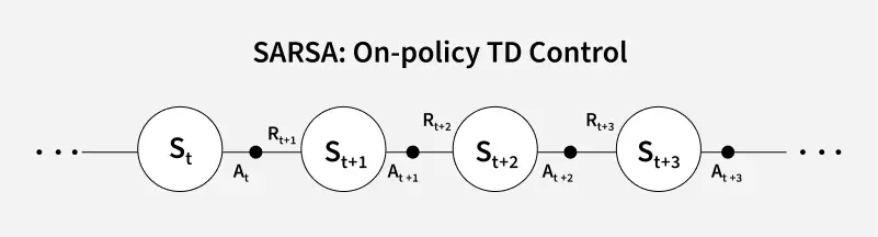
SARSA (On-Policy TD Control)

SARSA learns action-value function Q(s, a) for the current behavior policy (typically ε-greedy). Its update rule incorporates the next action selected by the same policy:

Q(S_t, A_t) \leftarrow Q(S_t, A_t) + \alpha \left[ R_{t+1} + \gamma Q(S_{t+1}, A_{t+1}) - Q(S_t, A_t) \right]

• On-policy: Updates Q -values using actions actually taken during exploration.
• Convergence: Learns the value of the exploration-influenced policy.
• Risk aversion: In stochastic environments, SARSA may learn safer policies by accounting for exploration noise.

Q-Learning (Off-Policy TD Control)

Q-learning directly approximates the optimal action-value function q^* independent of the behavior policy:

Q(S_t, A_t) \leftarrow Q(S_t, A_t) + \alpha \left[ R_{t+1} + \gamma \max_{a} Q(S_{t+1}, a) - Q(S_t, A_t) \right]

• Off-policy: Uses a greedy target (\max_{a} Q ) while following an exploratory policy.
• Optimality: Converges to the optimal policy under standard conditions.
• Flexibility: Decouples exploration (behavior policy) from learning (target policy).