Xavier initialization

Xavier initialization is a technique used to initialize the weights of neural network which solves the problem of vanishing and exploding gradients which can hinder the training of deep neural networks. In this article, we will explore the significance of Xavier initialization, its mathematical foundation and why it plays a pivotal role in training deep neural networks.

Understanding Xavier Initialization

Xavier initialization is named after Xavier Glorot, who introduced this method in a 2010 paper co-authored with Yoshua Bengio. In their influential research paper titled "Understanding the Challenges of Training Deep Feedforward Neural Networks," the authors conducted experiments to investigate a widely accepted rule of thumb in the field of deep learning. This rule involves initializing the weights of neural networks by selecting random values from a uniform distribution that ranges between -1 and 1. After this random initialization, the weights are then scaled down by a factor of 1 divided by the square root of the number of input units (denoted as 'n').

It aims to address the issue of maintaining variance in the forward and backward passes of a neural network, specifically when using certain activation functions like the hyperbolic tangent (tanh) and the logistic sigmoid. Regardless of how many input connections a neuron in a layer has, the variance of its output should be roughly the same. This property helps to prevent the vanishing or exploding gradient problem which can occur if the variances change drastically between layers. Similarly the variance of the gradients during backpropagation should also be roughly constant regardless of the number of neurons in the subsequent layer. This helps in maintaining stable training dynamics.

In Xavier initialization, key factor is the number of inputs and outputs in the layers and not so much the method of randomization. Goal is to maintain the variance in bounds that enable effective learning with various activation functions.

Uniform Xavier Initialization

We can initialize the weights by drawing them from a random uniform distribution within a specific range which is determined by the formula:

x = \sqrt {\frac {6}{n_{inputs}\,+\,n_{outputs}}}

• x is calculated using above formula.
• n_{inputs} : Number of Input in the input layer
• n_{output} : Number of Output in the Output layer

For each weight in network we draw a random value w from a uniform distribution in the range [-x, x].

By constraining the weights within a range determined by x , you ensure that the variance of the initial weights is controlled and is suitable for effective training.

Normal Xavier Initialization

This initialization sets the initial weights by drawing them from a gaussian distribution with a mean of 0 and a specific standard deviation, which is determined by the formula:

\sigma = \sqrt {\frac {2}{n_{inputs}\,+\,n_{outputs}}}

• \sigma is calculated using the provided formula
• n_{inputs} : Number of Input in the input layer
• n_{output}: Number of Output in the Output layer

For each weight in the network, draw a random value w from a normal distribution with mean 0 and standard deviation σ. Assign this random value as the initial weight for that connection. By setting the standard deviation based on the number of inputs and outputs, it adjusts the scale of the weights in a way that keeps the network's activations within a reasonable range, regardless of the layer size.

Choice between Normal Xavier initialization and Uniform Xavier initialization may depend on the specific neural network architecture and the activation functions used.

Importance of Weight Initialization

Before diving into Xavier's initialization let's talk about the significance of initialization in deep learning.

1. Vanishing and Exploding Gradient: Problem of vanishing gradients occurs when gradients during training become extremely small causing the network to learn very slowly or not at all particularly in deep networks. On the other hand the problem of exploding gradients happens when gradients become extremely large, leading to unstable and ineffective training often causing the model to diverge. Both issues can hinder the successful training of deep neural networks.
2. Problem of Overfitting: Neural networks particularly deep ones have a high capacity to learn complex patterns from data. However this capacity also makes them prone to overfitting. Weight initialization indirectly helps tackle overfitting by ensuring that the neural network starts training with well-scaled weights which prevents issues like vanishing gradients and neuron saturation.
3. Saturation: Saturation of activation functions refers to a situation where the output of an activation function becomes extremely close to its minimum or maximum value for a wide range of inputs. In this state activation function becomes insensitive to changes in its input and its gradient approaches zero. By setting the initial weights appropriately weight initialization helps keep activations in a balanced range preventing saturation and associated gradient problems.

Python Implementation

Below is a step-by-step explanation of the code:

1. Import Necessary Modules

Here we will use numpy, keras and tenserflow. Sequential model allows you to create a linear stack of layers and other modules are used to define different types of layers in the model.

import tensorflow as tf
from tensorflow.keras import layers, models
from tensorflow.keras.datasets import mnist
import numpy as np

2. Loading the dataset

Here we used mnist dataset for model training.

• train_images, test_images = train_images / 255.0, test_images / 255.0: Normalizes the image data by scaling the pixel values which range from 0 to 255 to a range between 0 and 1. This is done by dividing each image’s pixel values by 255.0.

(train_images, train_labels), (test_images, test_labels) = mnist.load_data()
train_images, test_images = train_images / 255.0, test_images / 255.0

3. Building a simple neural network

In the following code snippet we have defined a simple neural network with Xavier Initialization.

• Input layer is a Flatten layer, which is used to flatten the 28x28 input images into a 1D array.
• We have defined two dense layer with 128 and units, ReLU activation and Xavier initialization for weight initialization.
• Output layer consists of 10 units (for the 10 classes in the MNIST dataset) and uses the softmax activation function. Again, Xavier Initialization is applied to the weights.

model = models.Sequential()
model.add(layers.Flatten(input_shape=(28, 28)))

model.add(layers.Dense(128, kernel_initializer='glorot_uniform', activation='relu'))
model.add(layers.Dense(64, kernel_initializer='glorot_uniform', activation='relu'))

model.add(layers.Dense(
    10, kernel_initializer='glorot_uniform', activation='softmax'))

model.compile(optimizer='adam',
              loss='sparse_categorical_crossentropy',
              metrics=['accuracy'])

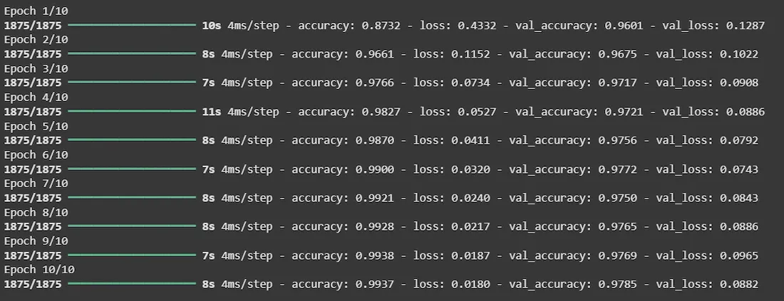
4. Model Training

Here we will be training model on 10 epochs.

history = model.fit(train_images, train_labels, epochs=10,
                    validation_data=(test_images, test_labels))

Output:

5. Model Evaluation

test_loss, test_acc = model.evaluate(test_images, test_labels)
print(f'Test accuracy: {test_acc * 100:.2f}%')

Output:

Test accuracy: 97.85%

Use Case

Xavier Initialization uses a factor of 2 in the numerator when initializing weights for activation functions like sigmoid and tanh because these functions have derivatives that are relatively small compared to the linear activation functions. Let's break down why this factor is used:

1. Sigmoid Activation

Sigmoid activation function squeezes its input into the range [0, 1]. For inputs that are far from zero derivative of the sigmoid function becomes very small, approaching zero. This means that during backpropagation gradients can vanish when weights are initialized too large making training difficult. Factor of 2 in Xavier Initialization helps counteract this effect by ensuring that the variance of the weights is appropriate to prevent the gradients from vanishing too quickly.

2. Hyperbolic Tangent (tanh) Activation

Tanh activation function also compresses its input into a range between -1 and 1. Similar to sigmoid, the tanh function has derivatives that become very small as inputs move away from zero. Therefore without proper initialization, gradients can vanish during training. Factor of 2 in Xavier Initialization addresses this issue by controlling the variance of the weights, making it easier to train networks with tanh activation functions.

In both cases factor of 2 helps balance the initialization such that the weights are neither too small (leading to vanishing gradients) nor too large (leading to exploding gradients). Xavier Initialization aims to provide a suitable starting point for training by ensuring that the gradients are not too small for efficient learning.