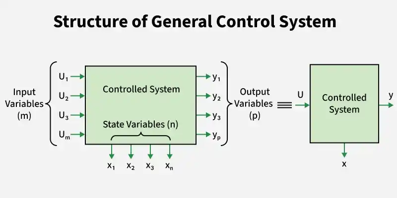
A Control System is a system or a set of devices that manages, commands, and directs the behavior of other devices or systems. It consists of three main components: a sensor, a controller, and an actuator.
- Sensor: Measures physical quantities like temperature, speed, or pressure and converts them into signals for the control system.
- Controller: Compares the measured value with the desired value and generates a control signal to reduce the error.
- Actuator: Receives the control signal and produces physical action, such as moving a motor or opening a valve.
Importance of Control System
- Enhances system stability and reliability.
- Reduces the effect of disturbances and external changes.
- Enables automation, reducing human effort and errors.
- Improves accuracy and maintains the desired output of a system
- Enhances the efficiency, safety, and performance of machines and processes.
Classification of Control Systems
Based on the type of signal used and operate
- Continuous signal - Control signals are continuous with respect to time.
- Discrete signal - Consists of more discrete signals.
Based on the Number of inputs and Output Present
- SISO - Single Input Single Output, it consists of one input and one output.
- MIMO - Multiple Input Multiple Output, which consists of two or more inputs to give outputs.
Based on the Feedback Path
- Open loop control system - Control action is not dependent of desired output and it requires human efforts to operate.
- Closed loop control system - Control action is dependent of output and input is applied to controller processes it to give signal.
Open-Loop Control System:
In an open-loop controlled system a control signal which is considered input is sent to a system (Source), and the system responds without considering the output.
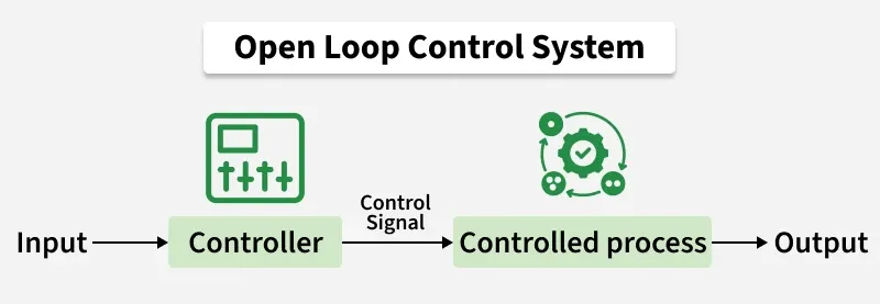
Examples of Open-Loop Control Systems:
- Washing machine with preset timer
- Electric toaster
- Electric hand dryer
- Automatic sprinkler system (timer-based)
Closed-Loop Control System:
Closed-loop control system sensors used to provide system performance and then adjust the control input accordingly. This system is also called feedback control system.
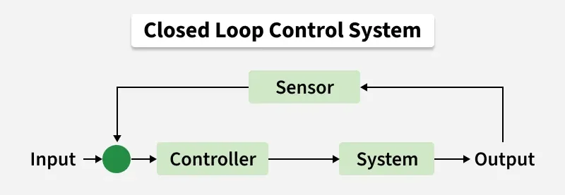
Examples of Closed-Loop Control Systems:
- Automatic temperature control system (e.g., air conditioner, refrigerator)
- Speed control system of a motor
- Water level control system in tanks
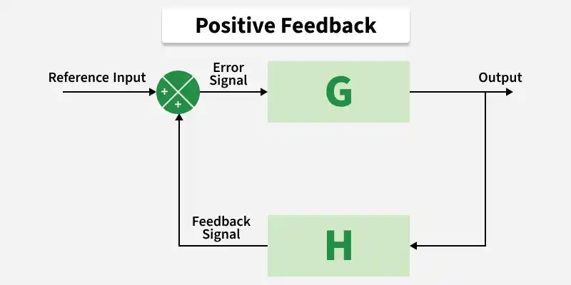
Feedback
Feedback is the process of sending some portion of the output signal back to the input of the system.
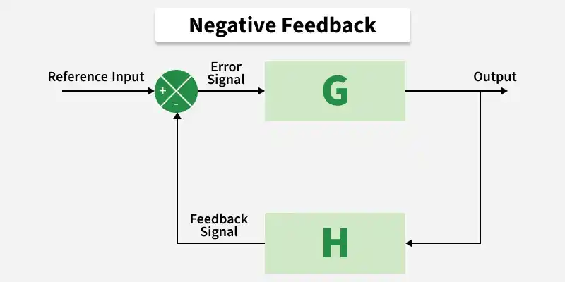
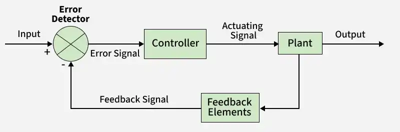
Components of a Feedback Control System
- Reference Input (Command Input): The desired value applied to the system.
- Output: The actual response of the system.
- Feedback Path: Returns a portion of the output to the error detector for comparison.
- Error Detector: Compares the reference input with the feedback signal and produces the error (actuating signal).
- Controller: Processes the error signal and generates a control action.
There are two types of feedback: Positive Feedback and Negative Feedback
Positive Feedback
The input signal is the sum of the actual signal, and the feedback signal is known as positive feedback.
The Transfer Function of Positive FeedBack Written as:
Example:
Audio Microphone Speaker System: Sound from the speaker re-enters the microphone, amplifies further, and causes howling or squealing.
Negative Feedback
The input signal is the difference between the original input and the feedback signal that signal is known as negative feedback.
The Transfer Function of Negative FeedBack Written as:
Example:
Automatic Voltage Regulator (AVR): It maintains constant output voltage by correcting variations using feedback.
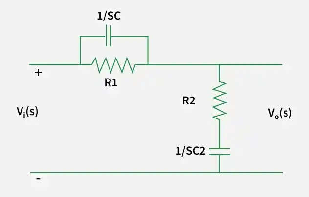
Transfer Function
The Transfer Function is the ratio of laplace transform of output to laplace transform of input with all initial conditions assumed to be zero.
Transfer function G(s) :
Laplace Transform
The Laplace transform of a time-domain function f(t)f(t)f(t) is defined as:
It converts a time-domain signal into the s-domain.
Laplace Transform is Used in Control Systems
- Converts differential equations into algebraic equations
- Simplifies analysis of Linear Time-Invariant(LTI) systems
- Helps in handling initial conditions
- To define and analyze the transfer function
Standard Laplace Transforms
Laplace Transform of Derivatives
First derivative:
Second derivative:
Transfer Function of OLTF and CLTF
1. Open-Loop Transfer Function (OLTF)
The open-loop transfer function is the product of the transfer functions of all components in the forward path of the system, without feedback.
Where:
G(s) = Forward path transfer function
H(s) = Feedback path transfer function
If no feedback is considered:
2. Closed-Loop Transfer Function (CLTF)
The closed-loop transfer function is the ratio of the output to the reference input when feedback is present.
For Positive Feedback:
For Negative Feedback:
Block Diagram
A block diagram is a graphical representation of a control system in which each component is represented by a block showing its transfer function, and the blocks are interconnected to depict the flow of signals and their relationships within the system.
Basic Elements of Block Diagram
- Functional Block: This symbol represents the transfer function G(s) of a system.
- Summing Point: This is the point where different output signals from the previous block or different signals of the system are added to form a single signal
- Take Off Point: It is a tapping point in the system where the desired signal is tapped off to be utilized elsewhere in the diagram.
Transfer Function For Block Diagram
The transfer function of a control system is obtained by reducing its block diagram step by step.
- R(s) = input
- C(s) = output
Steps to Find Transfer Function from a Block Diagram
Identify individual blocks: Write the transfer function of each block in the diagram.
Combine blocks in series (cascade): Multiply their transfer functions.
Combine blocks in parallel: Add or subtract their transfer functions
Reduce feedback loops
For a feedback system:
For Positive Feedback,
For Negative Feedback,
Repeat the reduction: Continue simplifying until a single block remains between input and output.
Block Diagram Reduction
Block Diagram Reduction Technique in used to analyze and simplify the complex system represented by block diagram. A block diagram of a system is a pictorial representation of the the function performed by each component and of the flow of signals.
Objectives of Block Diagram Reduction
1) System Analysis
- Block diagrams represent the interconnections and relationships between system components.
- They help engineers understand component interactions and predict overall system behavior.
2) Simplification
- Reducing complex systems makes them easier to understand and analyze.
- Simplified diagrams improve visualization and make communication clearer.
3) Design and Synthesis
- Reduction allows modification of the system structure during design.
- Engineers can optimize the system for desired performance and control objectives.
4) Control System Stability Analysis
- Simplified diagrams help apply stability criteria to analyze system behavior.
- Stability analysis guides controller design and ensures predictable operation.
5) Troubleshooting and Debugging
- Reduction helps isolate faulty components or connections in the system.
- Enables systematic identification and resolution of problems for reliable operation.
Signal Flow Graph
A Signal Flow Graph (SFG) is a directed edge and node-based visual depiction of the dynamics of a system. SFGs are widely used in control theory because they provide an easy-to-understand representation of intricate system relationships, which helps with analysis and optimization.
Basic Elements of Signal Graph
Node
- A node represents a system variable (signal), such as input, output, or an intermediate variable.
- It denotes a point where signals are summed or distributed.
Source Node
- A node with only outgoing branches and no incoming branches.
- Represents an independent input to the system.
Sink Node
- A node with only incoming branches and no outgoing branches.
- Represents the output of the system.
Branch
- A branch is a directed line connecting two nodes.
- It represents the functional relationship between the variables.
Branch Gain
- The transmittance associated with a branch.
- It indicates how the signal is multiplied as it passes from one node to another.
Path
- A sequence of connected branches followed in the direction of arrows.
- Shows how a signal travels from one node to another.
Forward Path
- A path from the source node to the sink node without passing through any node more than once.
- Used in Mason’s Gain Formula.
Feedback Loop
- A loop is a closed path that originates and terminates at the same node.
- No node is repeated more than once while tracing the loop.
Loop Gain
- The product of branch gains around a loop.
- Indicates the strength of feedback.
Non-touching Loops
- Loops that do not share any common nodes.
- Important in calculating the overall system transfer function using Mason’s Gain Formula.
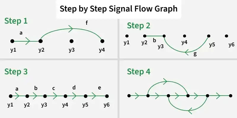
Step by Step Signal Flow Graph
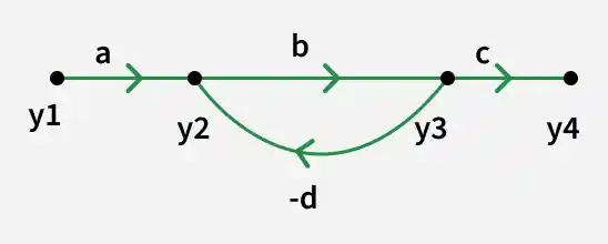
Equations:
Here, "y1, y2, y3, y4, y5, y6" are the nodes, and "a, b, c, d, e, f, g" are the gains in the Signal Flow Graph respectively.
- Step1: Create the first loop, and required branches with the y2 and y4 equation.
- Step2: Create the second loop, and don't forget the directions with the y3 equation, we have to be careful with the directions. Give directions according to the equations.
- Step3: Create the main branch with directions, and connect all the nodes with branches.
- Step4: Now we have to combine the whole structure and we will get the whole Signal Flow Graph, with proper notations and directions.
Mason’s Gain Formula
In the Signal Flow Graph (SFG) approach, once the SFG is obtained, the overall system transfer function can be directly evaluated using Mason’s Gain Formula.
Where:
- K = Number of forward paths
- Pk = Gain of the k^{th} forward path
- Δ(Delta)= Graph Determinant
Δk(\Delta_k) = Cofactor of the graph determinant for the kth forward path
Time Response
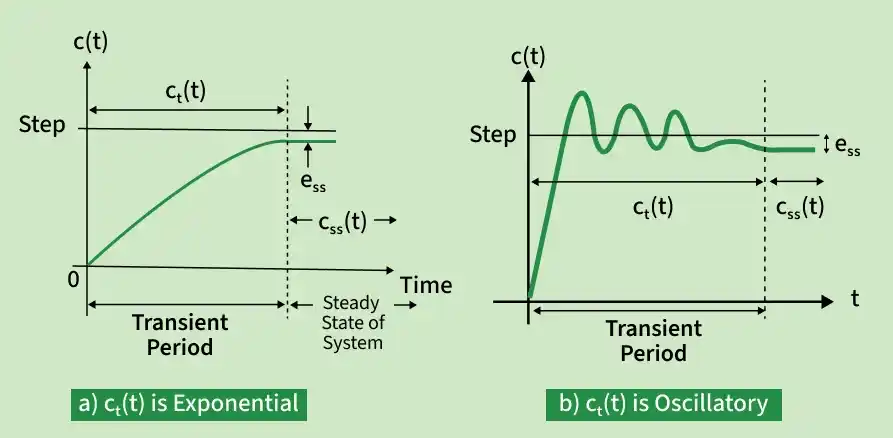
The Response of the system as a function of time, to the applied excitation is called Time Response. The steady-state response and transient response are two components of the total response of a control system. Their sum is equal to the total response.
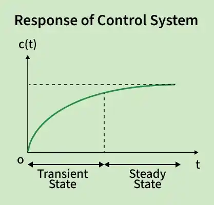
Steady-State Response: The steady-state response is the part of the total response that does not approach zero as time approaches infinity (
Transient Response: The transient response is that approaches zero as time approaches infinity (
The time response of a control system can be expressed as the sum of its transient response and steady-state response:
Where,
Time Domain Analysis is the study of a control system response with respect to time for standard inputs like step, ramp, and impulse.
Type and Order of a System
- Type: The number of open loop poles at origin (s=0) is the type of system.
- Order: Total number of open loop poles is the order of closed loop system.
First Order System Response
System with only one pole is called as first order system.
The transfer function as,
Where,
Therefore,
This equation gives the speed of response of system for an input. Higher the time constant, slower is the response and vice-versa.
Order | Input Type | Equation |
|---|---|---|
1 | Impulse | |
1 | Unit Step | |
1 | Ramp |
Second Order System
The systems with two poles are called second order systems. The transfer function for second order system is
Where,
\omega_n : System Natural Frequency. It is the frequency at which the system tends to oscillate in the absence of damping force.\epsilon : System Damping Ratio. It is a dimensionless quantity describing decay of oscillations during transient response.- System damped frequency(
\omega_d ) is the frequency at which the system tends to oscillate in presence of damping force.\omega_d = \omega_n \sqrt{1 - \epsilon^2}
Response Analysis of Second order system
| Sr. No. | Range of ξ | Types of Closed Loop Poles | Nature of Response | System Classification |
|---|---|---|---|---|
| 1 | ξ > 1 | Real, unequal & negative | Purely exponential | Overdamped |
| 2 | ξ = 1 | Real, equal & negative | Critically damped, pure exponential | Critically damped |
| 3 | 0 < ξ < 1 | Complex conjugate with negative real part | Damped oscillations | Underdamped |
| 4 | ξ = 0 | Purely imaginary | Oscillations with constant frequency and amplitude | Undamped |
Stability Analysis
The Stability of the system means when a controlled input is provided to any dyanamic system, it mucst result in providing the controlled output.
Types of Stability
1. Steady-State Stability: A system is steady-state stable if, for a constant input over a long time, the output settles to a finite constant value.
2. Transient Stability: Transient stability indicates whether the system remains stable during the transition period after a disturbance.
3. BIBO Stability: System is BIBO stable if every bounded input produces a bounded output.
Responses of SOS
Routh–Hurwitz Stability Criterion
It is a method that is used to determine the stability of the linear time-invariant (LTI) system. It provides information about the roots in the right half of the s-plane by analyzing the coefficients of the characteristic equation of the system.
According to the Routh Hurwitz Criteria, the polynomial must satisfy the following 3 conditions:
- All coefficients of the polynomial must have same sign.
- All the terms in first column of the Routh's Array must have the same sign.
- All the power of 's' must be present in the characteristic equation.
The Routh–Hurwitz stability criterion uses this characteristic equation to determine system stability without solving for roots.
Example:
Examine the stability of given equation using Routh’s method
Creating the Routh’s Array:
| Power of s | First Column | Second Column |
|---|---|---|
| 1 | 3 | |
| 2 | 6 | |
| 0 | ||
| 6 | — |
Rules of Routh–Hurwitz Stability Criterion
Rule 1: For a system to be stable, all elements of the first column of the Routh table must be positive and non-zero.
Rule 2: If the first element of any row is zero (but the row is not all zeros):
- Indicates at least one root on the Right Half Plane (RHP)
- The system becomes UNSTABLE
Rule 3: Row of Zeros (Below Auxiliary Equation – AE)
A row of zeros indicates the presence of symmetrical roots about the origin.
| Case | Sign of Δ | Nature of Roots | Location of Roots |
|---|---|---|---|
| 1 | Sign change | Symmetric real roots | Right Half Plane (RHS) |
| 2 | No sign change | Symmetric imaginary conjugate roots | Imaginary axis |
| 3 | Repeated | Repeated symmetric roots | LHS + RHS |
| 4 | Repeated | Repeated imaginary roots | Imaginary axis |
In this case, form the Auxiliary Equation (AE) from the row above and differentiate it to continue the Routh array.
Rule 4: If there is a sign change in the first column above the AE:
Number of sign changes = Number of roots in RHS of the s-plane
Root Locus
The root locus is a graphical method used in control system design to study how the closed-loop poles of a system move when a parameter, usually a gain, is changed.
- Number of root locus branches = number of open-loop poles.
- Root locus starts at open-loop poles (K=0).
- Root locus ends at open-loop zeros (
K \to \infty ). - If poles > zeros, extra branches go to infinity along asymptotes.
- Root locus is symmetrical about the real axis.
- Used mainly for stability analysis and controller design.
Step-by-Step Procedure for Creating Root Locus Plot
Step 1: Start with Open-Loop Transfer Function
Use
Step 2: Determine Characteristic Equation
Use 1 + KG(s) = 0 to study closed-loop behavior
where,
- K is the control parameter (gain of a controller).
- G(s) is the open-loop transfer function.
Step 3: Identify Open-Loop Poles and Zeros
- Poles: roots of D(s)=0
- Zeros: roots of N(s)=0
- These are starting/ending points of the locus.
Step 4: Determine Number of Branches
Equal to the number of open-loop poles; each branch starts at a pole.
Step 5: Calculate Breakaway & Break-in Points
Solve
Step 6: Determine Asymptotes
- Number: Poles − Zeros
- Angle:
\theta_a = (N - P)(2n + 1)\pi , n = 0, 1, ...., N-P-1 - Centroid:
\text{Centroid} = \frac{\sum \text{Poles} - \sum \text{Zeros}}{N - P}
Step 7: Draw the Root Locus
Start at poles, follow branches toward zeros/asymptotes as K increases.
Step 8: Check for Imaginary Axis Crossing
Determines stability; occurs when poles cross imaginary axis.
Step 9: Calculate Gain for Desired Pole Locations
Select desired closed-loop pole positions (damping, frequency) and find K from plot.
Step 10: Evaluate Performance
Analyze overshoot, settling time, and transient response for selected K.
Nyquist Stability Criterion
The Nyquist Stability Criterion is a frequency-domain method used to determine the stability of a closed-loop control system by analyzing the open-loop transfer function.
Key Terms
- P: Number of open-loop poles in the right half s-plane (RHP).
- N: Number of clockwise encirclements of the point (−1,0).
- Z: Number of closed-loop poles in the RHP.
Principle of Argument in Nyquist Plot
If a transfer function has P poles and Z zeros enclosed by a contour in the s-plane, then the corresponding Nyquist (GH-plane) contour encircles the origin (Z−P) times.
Z > P \;\Rightarrow\; N = Z - P > 0 → Clockwise encirclement of (−1,0)(-1,0)(−1,0) → Unstable systemP > Z \;\Rightarrow\; N = Z - P < 0 → Anti-clockwise encirclement → Stable systemZ = P \;\Rightarrow\; N = 0 → No net encirclement → Marginally stable system
Important Terminologies of Nyquist Plot
1. Nyquist Path / Contour
- A closed contour in the s-plane that encloses the entire right half plane.
- It is mapped into the GH-plane to study system stability.
2. Nyquist Encirclement
- Refers to how many times the Nyquist plot encircles the critical point (−1,0).
- Direction of encirclement (clockwise or anti-clockwise) determines system stability.
3. Nyquist Mapping
- The process of mapping the Nyquist contour in the s-plane into the GH-plane.
- Used to apply the Principle of Argument for stability analysis.
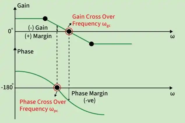
4. Gain Crossover Frequency (
- Frequency at which the magnitude of open-loop transfer function equals unity (
\lvert G(j\omega)H(j\omega) \rvert = 1 ). - Used to calculate the Phase Margin.
5. Phase Crossover Frequency (
- Frequency at which the phase angle of
G(j\omega) H(j\omega) is −180°. - Used to determine the Gain Margin.
6. Phase Margin (PM)
- Additional phase lag required at
\omega_{gc} to bring the system to instability. - Indicates relative stability of the control system.
7. Gain Margin (GM)
- Factor by which system gain can be increased before the system becomes unstable.
- Measured at the phase crossover frequency
\omega_{pc} .
Bode Plot
A Bode plot is a graphical representation of a linear time-invariant system in the frequency domain. It consists of two plots:
- Gain plot: Shows gain (
|G(jω)| ) vs frequency (ω) in dB. - Phase plot: It shows phase (
∠G(jω) ) vs frequency (ω) in degrees.
Compensator
A device inserted into the system for the purpose of satisfying the specifications such as stability, accuracy, and speed of response is called a compensator.
There are three types of Compensator:
- Lead Compensator
- Lag Compensator
- Lag-lead Compensator
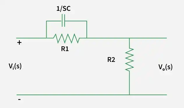
Lead Compensator
Lead Compensator is used to increase phase margin, making the system faster and more stable.
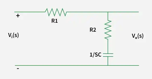
Lag Compensator
Lag compensator is used to reduce steady-state error by increasing low-frequency gain, with little effect on transient response.
Lead vs Lag Compensator
| Performance Parameter | Lead Compensator | Lag Compensator |
|---|---|---|
| Speed of response | ↑ (Increases significantly) | ↓ (Decreases) |
| Damping ratio (ζ) | ↑ (Improves damping) | ↓ (Slight reduction) |
| Bandwidth (BW) | ↑ (Increases significantly) | ↓ (Decreases) |
| Stability | ↑ (Improves stability) | Slight ↑ (Marginal improvement) |
| Steady-state error (eₛₛ) | Slight ↓ | ↓ (Reduces significantly) |
| Maximum peak (MP) | ↓ (Reduces overshoot) | ↑ (May increase overshoot) |
| Oscillations | ↓ (Less oscillatory) | ↑ (More oscillatory) |
| Gain margin (GM) | ↑ (Large improvement) | Slight ↓ or almost same |
Lag-Lead Compensator
Lag–Lead compensation is a combination of lag and lead compensators to achieve accuracy and speed together.
Applications of Compensators
- To improve system stability by increasing phase and gain margins
- Reduce steady-state error and improve accuracy
- Enhance transient response (reduce rise time, settling time, and overshoot)
- Increase bandwidth of the control system
- Stabilize unstable or marginally stable systems
- Used in servo systems, industrial process control, aerospace, and robotic control systems
Controller
The controller is a critical component used to regulate the behavior of dynamic system or process. The Controllers are essential for maintaining desired performance and accuracy in various engineering and automation applications.
Example:
Cruise Control in Vehicles:
The cruise control is a classic example of a closed-loop control system. The driver sets a desired speed and controller adjusts the throttle or engine power based on feedback from the speed sensors to maintain the set speed.
- Speed Sensor: Measures the actual vehicle speed.
- Reference Speed: Represents the desired speed set by driver.
- Error Calculation: Computes the speed error.
Applications of Controllers
- Industrial Automation: The Controlling processes in manufacturing and industrial machinery.
- Aerospace: The Managing flight systems, autopilots and navigation.
- Automotive: To Implementing cruise control or anti-lock braking systems and engine control units.
- Robotics: The Regulating robot movements and autonomous navigation.
- Home Automation: The Controlling heating, ventilation and smart devices.
Types of Controllers
- Proportional (P) Controller: Produces a control signal proportional to the present error, reducing rise time but not eliminating steady-state error.
- Integral (I) Controller: Generates control action based on accumulated past error, eliminating steady-state error but slowing response.
- Derivative (D) Controller: Acts on the rate of change of error, improving stability and damping by predicting system behavior.
State Space Analysis
State Space Analysis is the graphical tool that is used to analyze and design the linear, non-linear, time-variant, time-invariant multi-input, multi-output system.
There are various key components of the state space analysis which are as follows:
- State: The minimum information needed to describe the system at any time.
- State Variables: Set of variables that define the state of the system.
- State Vector: A vector formed by state variables.
- State Equation: First-order differential equation describing system dynamics.
- Output Equation: An equation relating state variables to the output.
- State Space Representation: Mathematical model using state and output equations.
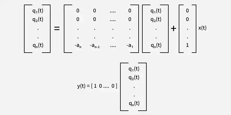
State Variable Model
A state-space (state variable) model represents a system using first-order differential equations in terms of state variables.
General State-Space Representation
where,
- q(t) = State vector
\dot{q} = Time derivative of state vector- u(t) = Input vector
- y(t) = Output vector
- A = System matrix
- B = Input matrix
- C = Output matrix
- D = Feed-through (or direct transmission) matrix
Example on State Space Analysis
Example: Obtain the state space equation of the following differential equation:
Solution:
Triple derivative --> 3 variables
Controllability
A system is said to be controllable if it is possible to drive the state of the system from any initial state to any desired final state in finite time using a suitable control input.
The controllability matrix is:
Condition
- If
\operatorname{rank}(Q_c) = n then the system is controllable. - If
\operatorname{rank}(Q_c) < n then the system is uncontrollable.
Q0 = [B AB A2B ..... An-1B]
If the determinant of Q0 is not equal to 0 then the system is controllable.|Q_0| \neq 0 ---- (System is controllable)\lvert Q_0 \rvert = 0 ----- (System is uncontrollable)
Observability
A system is said to be observable if the initial state of the system can be completely determined from the input and output measurements over a finite time interval.
Q0 = [CT ATCT ..... (AT)n-1CT]
If the determinant of Q0 is not equal to 0 then the system is controllable.|Q_0| \neq 0 ---- (System is observable)\lvert Q_0 \rvert = 0 ----- (System is not observable)
