How to Make a Budget Spreadsheet in Google Sheets

Creating a budget spreadsheet is an essential skill for managing personal finances, and Google Sheets offers a versatile platform to make this task easy and efficient. Whether you’re new to budgeting or looking to streamline your financial tracking, learning how to make a budget spreadsheet in Google Sheets can help you stay organized and achieve your financial goals.

1. How to Create a Budget Spreadsheet in Google Sheets

Budget spreadsheets can be made from many methods. Methods to create a budget spreadsheet are as follows:

• Creating Budget Spreadsheet manually
• Creating Budget Spreadsheet by downloading Templates

2. How to Make a Budget Spreadsheet manually

Step 1: Open Google Sheets

Open Google Sheets by searching it on your desired browser.

Step 2: Create a new spreadsheet

Create a new spreadsheet by clicking on blank or you can also open pre-existing document also.

Step 3: Enter your data

Choose a cell and a row and enter all your data manually.

Step 4: Edit the data

Edit your data so that your spreadsheet looks pretty using different tools in tool bar.

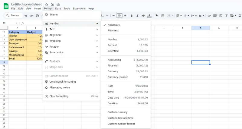
Step 5: Change numbers to currency

You should change your numbers to currency as it is a budget spreadsheet, so currency is important. you can do so by clicking on format then numbers and then selecting currency.

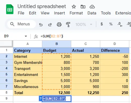
Step 6: Use simple formulae

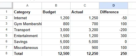
Use simple formulae to perform sum and difference in the spreadsheet. You can use =SUM(cell address) to do the sum.

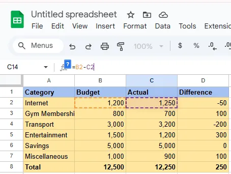
Step 7: Use simple difference formula

You can do difference in the spreadsheet by using =B2(cell address1) - C2(cell address2)

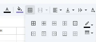
Step 8: Add borders

Adding borders to your spreadsheet may help it to be more effective. You can add borders by selecting the spreadsheet and then clicking on the 'borders' icon in tool bar.

Step 9. Conditional formatting

You need to know when you go under budget or over budget, Conditional formatting is the tool in google sheets application that helps you to do the same by giving different colours when you go under or over budget.

You can apply conditional formatting to your spreadsheet by clicking on Format then Conditional Formatting then select the range and edit the less than and color or more than and color option.

Your budget spreadsheet is now ready. and you can now save it to your storage.

3. How to Make a budget spreadsheet using downloaded templates

You can Download different spreadsheets template online. There are many budget spreadsheets template you may download online however, Google sheets themselves provide us with the budget spreadsheet templates.

Step 1: Open Google Sheets

Open google sheets from your google drive account.

Step 2: Select Monthly Annual or Quarterly Budget.

Select monthly budget, yearly budget or quarterly budget template that suits you.

Step 3: Use formulas.

Use easy formulae to perform calculations or to calculate your income, expense and balance.

Step 4: Edit the values.

Input your numbers and regularly update them.

Note: Some of the best spreadsheet-based applications are Google Sheets, Microsoft excel (MS Excel), LibreOffice Calc and OpenOffice.org Calc.

4. Uses of Spreadsheets

• We use spreadsheets to arrange data in rows and columns so that we can easily compare the data.
• spreadsheets are also useful in performing calculations in table form.
• We can also use spreadsheets to sort and store information.
• We use spreadsheets to track grades, budgets or inventory.

5. Some Basic google sheets formulae that can help you to perform budgeting:

• Budgeting can't be done without basic arithmetic operations that is multiplications, addition, subtraction and division.
• To get the total of a row or a column, we can use SUM formula (for example [ =SUM(B2:B10) ]the sheet application will do the sum of the B2 to cell B10).
• To get the sum of the range based on multiple criteria use SUMIFS formula [=SUMIFS(Sheet4!F:F,Sheet4!D:D,????ills”,Sheet4!E:E,”Person 1″) ]
• To get the average of a column or row, use the AVERAGE formula, such as =AVERAGE(B2:B10).
• To get the running balance of your income and expenses, use a formula that subtracts the withdrawals from the deposits in each row, such as =SUMIF(A$2:A2,"Deposit",B$2:B2)-SUMIF(A$2:A2,"Withdrawal",B$2:B2).