Stock prices may seem unpredictable, but they often follow patterns in data. By analyzing past prices and market indicators, we can build a machine learning model to forecast future movements. We will use CatBoost for Stock Prediction because:
- A gradient boosting algorithm that captures non-linear relationships in financial data.
- Automatically processes categorical variables without heavy preprocessing.
- Built-in techniques help improve model stability, which is critical for volatile markets.
- Faster experimentation and quicker model iteration.
- Delivers competitive accuracy compared to other boosting algorithms.

Implementation
Step 1: Importing required Libraries
Here we will import Pandas, Numpy, Matplotlib and Scikit Learn for its implementation.
import pandas as pd
import numpy as np
from catboost import CatBoostRegressor
from sklearn.model_selection import train_test_split
from sklearn.metrics import mean_squared_error
import matplotlib.pyplot as plt
Step 2: Load and Clean the Dataset
Download the dataset from here
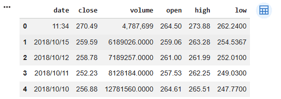
data = pd.read_csv("Your dataset path")
data.head()
Output:
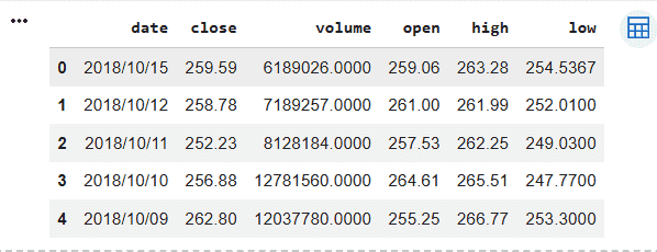
Step 3: Clean the Dataset
Remove incorrect rows and prepare the dataset for processing.
data = data.iloc[1:].reset_index(drop=True)

data.head()
Output:
Step 4: Convert Date Column and Sort Data
- Stock data must always be in time order.
- Sorting ensures the model learns from past and predicts future correctly.
data['date'] = pd.to_datetime(data['date'])

data = data.sort_values('date')
Step 5: Feature Engineering
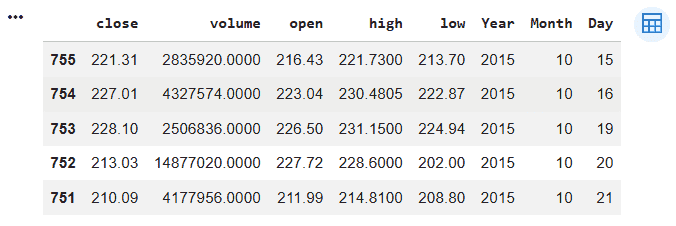
Machine learning models cannot directly understand dates. So we extract: Year, Month and Day
data['Year'] = data['date'].dt.year
data['Month'] = data['date'].dt.month
data['Day'] = data['date'].dt.day

data.drop(columns=['date'], inplace=True)

data.head()
Output:
Step 6: Define Features and Target
Separate input variables and output variable.
- X: Open, High, Low, Volume, Year, Month, Day
- y: Close price (what we predict)
X = data.drop(columns=['Close'])
y = data['Close']
Step 7: Time Based Train Test Split
We must split the data sequentially without shuffling; preserving time order which is important to prevent future data from leaking into the training process
split = int(len(data) * 0.8)

X_train = X[:split]
X_test = X[split:]

y_train = y[:split]
y_test = y[split:]
Step 8: Train CatBoost Model
The model learns patterns from historical stock data. CatBoost automatically handles feature relationships.
model = CatBoostRegressor(
    iterations=500,
    learning_rate=0.05,
    depth=6,
    verbose=0
)
model.fit(X_train, y_train)
Step 9: Make Predictions
Predict stock prices on unseen data.
y_pred = model.predict(X_test)
Step 10: Evaluate Model Performance
Measure how accurate the predictions are:
- RMSE shows average prediction error.
- Lower RMSE means better performance.
rmse = np.sqrt(mean_squared_error(y_test, y_pred))
print("RMSE:", rmse)
Output:
RMSE: 7.203
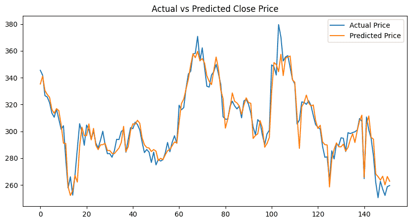
Step 11: Visualize Results
This helps visually compare:
- Real stock movement
- Model predictions
plt.figure(figsize=(10,5))
plt.plot(y_test.values, label="Actual Price")
plt.plot(y_pred, label="Predicted Price")
plt.legend()
plt.title("Actual vs Predicted Close Price")
plt.show()
Output:
Download full code from here
