Gradient Descent With RMSProp from Scratch

RMSprop modifies the traditional gradient descent algorithm by adapting the learning rate for each parameter based on the magnitude of recent gradients. The key advantage of RMSprop is that it helps to smooth the parameter updates and avoid oscillations, particularly when gradients fluctuate over time or dimensions.

The update rule for RMSprop is given by:

\theta_{new} = \theta_{old} - \frac{\eta}{\sqrt{E[\nabla_\theta J(\theta)]^2 + \epsilon}} \cdot \nabla_\theta J(\theta)

Key Steps of RMSprop:

• Compute the gradient: As in gradient descent, calculate the gradient of the objective function with respect to each parameter.
• Maintain an exponentially decaying average of the squared gradients: This helps adjust the step size dynamically for each parameter.
• Update parameters: Instead of using a fixed learning rate, RMSprop uses the moving average of the squared gradients to normalize the updates.

Implementation of RMSprop from Scratch

Let’s implement the RMSprop optimizer from scratch and use it to minimize a simple quadratic objective function.

1. Defining the Objective Function

We will begin by defining a simple quadratic objective function:

f(x_1, x_2) = 5x_1^2 + 7x_2^2

This function is convex and has a global minimum at x_1 = 0, x_2 = 0, which makes it an ideal candidate for demonstrating optimization techniques.

import numpy as np
import matplotlib.pyplot as plt
from numpy import arange, meshgrid

def objective(x1, x2):
    return 5 * x1**2.0 + 7 * x2**2.0
def derivative_x1(x1, x2):
    return 10.0 * x1
def derivative_x2(x1, x2):
    return 14.0 * x2

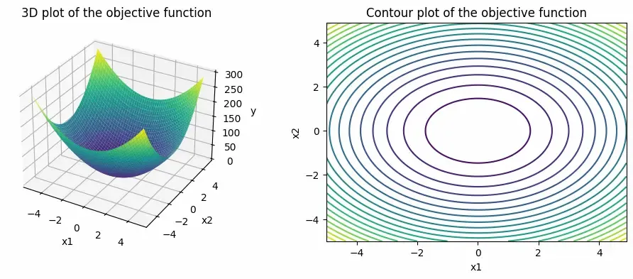
2. Visualizing the Objective Function

To better understand the optimization landscape, let's visualize the objective function using both a 3D surface plot and a contour plot.

x1 = arange(-5.0, 5.0, 0.1)
x2 = arange(-5.0, 5.0, 0.1)
x1, x2 = meshgrid(x1, x2)
y = objective(x1, x2)

fig = plt.figure(figsize=(12, 4))
ax = fig.add_subplot(1, 2, 1, projection='3d')
ax.plot_surface(x1, x2, y, cmap='viridis')
ax.set_xlabel('x1')
ax.set_ylabel('x2')
ax.set_zlabel('y')
ax.set_title('3D plot of the objective function')

ax = fig.add_subplot(1, 2, 2)
ax.contour(x1, x2, y, cmap='viridis', levels=20)
ax.set_xlabel('x1')
ax.set_ylabel('x2')
ax.set_title('Contour plot of the objective function')

plt.show()

Output:

3. Implementing RMSprop

Next, we’ll implement the RMSprop optimization algorithm. The algorithm will update the parameters x_1 and x_2​ iteratively by using the gradients and adjusting the learning rate dynamically.

def rmsprop(x1, x2, derivative_x1, derivative_x2, learning_rate, gamma, epsilon, max_epochs):
    x1_trajectory = []
    x2_trajectory = []
    y_trajectory = []

    x1_trajectory.append(x1)
    x2_trajectory.append(x2)
    y_trajectory.append(objective(x1, x2))

    e1 = 0
    e2 = 0

    for _ in range(max_epochs):
        gt_x1 = derivative_x1(x1, x2)
        gt_x2 = derivative_x2(x1, x2)
        e1 = gamma * e1 + (1 - gamma) * gt_x1**2.0
        e2 = gamma * e2 + (1 - gamma) * gt_x2**2.0

        x1 = x1 - learning_rate * gt_x1 / (np.sqrt(e1 + epsilon))
        x2 = x2 - learning_rate * gt_x2 / (np.sqrt(e2 + epsilon))

        x1_trajectory.append(x1)
        x2_trajectory.append(x2)
        y_trajectory.append(objective(x1, x2))

    return x1_trajectory, x2_trajectory, y_trajectory

4. Running the RMSprop Algorithm

Let’s now run the RMSprop algorithm for 50 iterations starting from an initial guess of x_1 = -4.0 and x_2 = 3.0.

x1_initial = -4.0
x2_initial = 3.0
learning_rate = 0.1
gamma = 0.9
epsilon = 1e-8
max_epochs = 50

x1_trajectory, x2_trajectory, y_trajectory = rmsprop(
    x1_initial,
    x2_initial,
    derivative_x1,
    derivative_x2,
    learning_rate,
    gamma,
    epsilon,
    max_epochs
)

print('The optimal value of x1 is:', x1_trajectory[-1])
print('The optimal value of x2 is:', x2_trajectory[-1])
print('The optimal value of y is:', y_trajectory[-1])

Output:

The optimal value of x1 is: -0.10352260359924752
The optimal value of x2 is: 0.0025296212056016548
The optimal value of y is: 0.05362944016394148

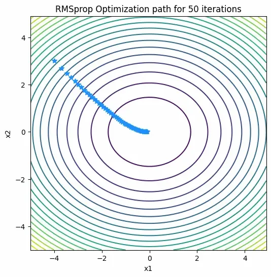
5. Visualizing the Optimization Path

Finally, we will plot the path taken by the RMSprop optimizer on the contour plot of the objective function to visualize how it converges to the minimum.

fig = plt.figure(figsize=(6, 6))
ax = fig.add_subplot(1, 1, 1)

ax.contour(x1, x2, y, cmap='viridis', levels=20)

ax.plot(x1_trajectory, x2_trajectory, '*',
        markersize=7, color='dodgerblue')

ax.set_xlabel('x1')
ax.set_ylabel('x2')
ax.set_title('RMSprop Optimization path for ' +
             str(max_epochs) + ' iterations')
plt.show()

Output:

The optimal values of x_1, x_2, and the objective function at the end of the optimization process. The plot shows the trajectory of the optimizer, indicating how the parameters gradually approach the minimum of the objective function.