Missing data imputation is the process of replacing missing or null values in a dataset with estimated values based on statistical or machine learning methods. It is an important step in data preprocessing since most machine learning algorithms cannot directly handle missing values, which may lead to errors, biased models or reduced performance.
- Essential for Model Training: Most ML algorithms like linear regression, SVMs and neural networks cannot process NaN values directly.
- Improves Data Quality: Imputation ensures datasets remain complete and consistent, allowing for better model accuracy.
- Model-Based Imputation: Techniques like IterativeImputer use predictive models to infer missing values based on observed data.
- Impact on Model Performance: Proper imputation minimizes data bias and preserves relationships within the dataset.
IterativeImputer
IterativeImputer is Scikit-learn’s implementation of multivariate imputation, designed to handle complex feature dependencies. It models each feature with missing values as a function of other features and iteratively refines the predictions.
Workflow
- Initialization: Missing values are first filled using a simple strategy like mean or median.
- Feature Selection: The algorithm selects a feature with missing values in a round-robin fashion.
- Model Training: A regression model predicts the missing values of that feature using the other features as predictors.
- Update: Imputed values replace the missing entries and the process continues for the next feature.
- Convergence: Iterations continue until values stabilize or the maximum number of iterations (max_iter) is reached.
This iterative cycle captures inter-feature dependencies, leading to more reliable imputations compared to univariate methods.
Implementation
The IterativeImputer algorithm has several key parameters that can be tuned for optimal performance:
- estimator: Base model used to predict missing values, by default it uses BayesianRidge()
- max_iter: The maximum number of iterations for the imputation process.
- tol: The tolerance threshold for convergence.
- n_nearest_features: The number of nearest features to use for imputation.
- initial_strategy: The initial imputation strategy, which can be either 'mean' or 'median'.
Step 1: Importing Necessary Libraries
We will import the required libraries such as numpy and scikit learn.
import numpy as np
from sklearn.experimental import enable_iterative_imputer
from sklearn.impute import IterativeImputer
from sklearn.datasets import make_regression
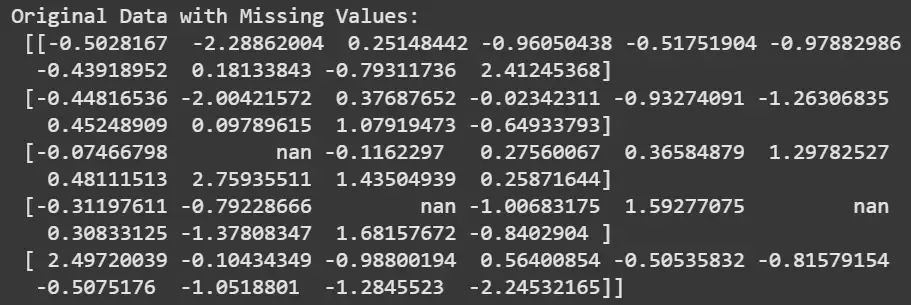
Step 2: Creating a Dataset with Missing Values
We will create a random dataset with missing values.
X, y = make_regression(n_samples=100, n_features=10, random_state=0)
mask = np.random.rand(*X.shape) < 0.1  # 10% missing values
X[mask] = np.nan

print("Original Data with Missing Values:\n", X[:5])
Output:
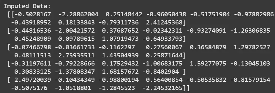
Step 3: Applying IterativeImputer
Now we will apply the IterativeImputer.
imputer = IterativeImputer(max_iter=10, random_state=0)
X_imputed = imputer.fit_transform(X)
print("\nImputed Data:\n", X_imputed[:5])
Output:
Choosing the Right Estimator
IterativeImputer allows flexibility in choosing the underlying estimator used for modeling missing features. The choice of estimator affects both accuracy and computational efficiency.
| Estimator | Description | Use Case |
|---|---|---|
| BayesianRidge | Linear regression with Bayesian regularization | Default choice for continuous features |
| DecisionTreeRegressor | Captures non-linear dependencies | Non-linear and complex datasets |
| ExtraTreesRegressor | Ensemble-based tree imputation | Large datasets with high variance |
| KNeighborsRegressor | Uses nearest neighbors for predictions | Small datasets with local patterns |
Advantages
- Higher Accuracy: Exploits correlations between multiple features for improved estimation.
- Flexible Architecture: Supports multiple estimators suited for different data distributions.
- Robustness: Handles both linear and non-linear relationships effectively.
Limitations
- Computationally Intensive: Iterative modeling can be slow for large datasets.
- Complex Configuration: Requires tuning of parameters such as iterations, estimators and convergence tolerance.
- Not Ideal for Sparse Data: Works best with continuous, dense data.
