In machine learning, it's important to understand how our models make decisions. SHAP values help explain these decisions, making them easier to understand. Here, we'll show you how to use SHAP values with an ElasticNet model, a type of regression model that combines two regularization methods.
What is ElasticNet?
ElasticNet is a type of linear regression that combines Lasso (L1) and Ridge (L2) regression. Lasso helps by setting some feature coefficients to zero, effectively selecting features. Ridge shrinks the coefficients of less important features but never to zero. Combining these helps handle datasets with many features or collinearity (highly correlated features).
What are SHAP Values?
SHAP (Shapley Additive explanations) values are a way to explain the output of machine learning models. They show how each feature contributes to the prediction. SHAP values ensure that the sum of the contributions of all features equals the prediction, providing a clear and consistent explanation.
Now we will discuss Step-by-step Implementation of How to Use SHAP on ElasticNet Machine Learning Model in R Programming Language.
Step 1: Load Necessary Libraries & Dataset
- glmnet for ElasticNet regression.
- MASS for the Boston housing dataset.
- iml for calculating and plotting SHAP values.
- Load the Boston dataset.
- Split the dataset into training and testing sets to validate the model's performance.
# Load the necessary libraries
library(glmnet)  # For fitting ElasticNet model
library(MASS)    # For the Boston housing dataset
library(iml)     # For calculating and plotting SHAP values

# Load the Boston housing dataset
data(Boston, package = "MASS")
X <- as.matrix(Boston[, -14]) # Predictor variables (all columns except the 14th)
y <- Boston[, 14]             # Response variable (the 14th column, MEDV)

# Split the data into training and testing sets
set.seed(42)  # For reproducibility
train_indices <- sample(1:nrow(X), nrow(X) * 0.8)
X_train <- X[train_indices, ]  # Training predictors
X_test <- X[-train_indices, ]  # Testing predictors
y_train <- y[train_indices]    # Training response
y_test <- y[-train_indices]    # Testing response
Step 2: Training the Model
Fit an ElasticNet model using cross-validation to find the optimal parameters.
# Train the ElasticNet model
# Perform cross-validated ElasticNet regression
model <- cv.glmnet(X_train, y_train, alpha = 0.5)
Step 3: Creating a Predictor Object
This is necessary for iml to calculate SHAP values. The predictor object is configured to work with the ElasticNet model's prediction function.
# Create a predictor object for the iml package
predictor <- Predictor$new(model, data = as.data.frame(X_train), y = y_train,
                           predict.fun = function(object, newdata) {
  predict(object, newx = as.matrix(newdata), s = "lambda.min")[,1]
})
Step 4: Calculating SHAP Values
Compute SHAP values for a single observation to understand the contribution of each feature to the model's prediction.
# Ensure the input data is correctly formatted as a data frame with correct dimensions
x_interest <- as.data.frame(X_test[1, , drop = FALSE])

# Calculate SHAP values for a single observation
shapley <- Shapley$new(predictor, x.interest = x_interest)
shapley$results
Output:
   feature         phi      phi.var feature.value
1     crim  0.54899182  1.833532345  crim=0.08829
2       zn  0.01305003  0.734931339       zn=12.5
3    indus  0.01808013  0.001029505    indus=7.87
4     chas -0.05855281  0.111972362        chas=0
5      nox  0.82755557  4.778691816     nox=0.524
6       rm -0.71419578  9.239779286      rm=6.012
7      age  0.02278470  0.005148661      age=66.6
8      dis -2.72742551  9.205870175    dis=5.5605
9      rad -1.16795643  5.982727995         rad=5
10     tax  0.99692882  2.610797043       tax=311
11 ptratio  3.14564086  4.930773768  ptratio=15.2
12   black  0.30031595  0.577063776   black=395.6
13   lstat  1.06359947 23.118524053   lstat=12.43
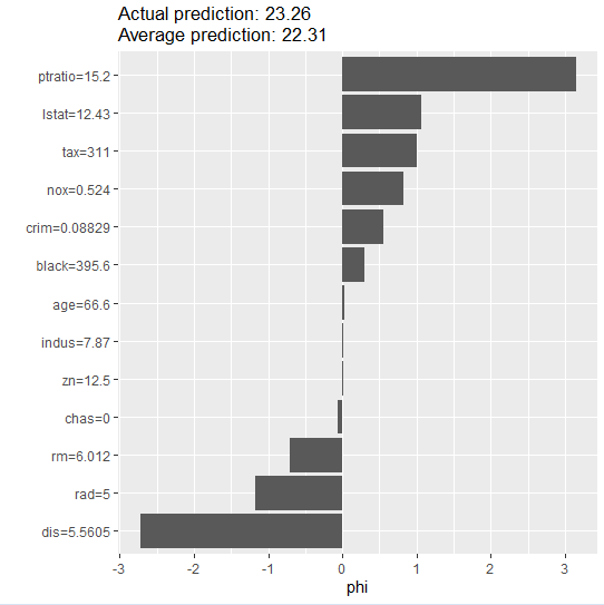
Step 5: Plotting SHAP Values
Plot these SHAP values to visualize feature contributions.
# Plot SHAP values for the single observation
shapley$plot()
Output:
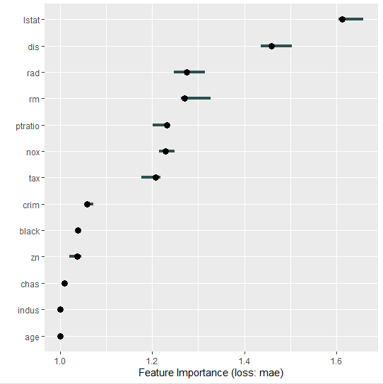
Step 6: Calculating Feature Importance
Compute and plot feature importance for the entire test set to understand which features are most significant in the model.
# Calculate feature importance for the entire test set
imp <- FeatureImp$new(predictor, loss = "mae")
plot(imp)
Output:
Conclusion
Using SHAP values to interpret an ElasticNet machine learning model is a powerful way to understand how different features contribute to predictions.This process helps in making our model more transparent and trustworthy, as it reveals the impact of each feature on the model's decisions. With these insights, we can improve our model, communicate findings more effectively, and make informed decisions based on the model's outputs.
