Seasonality Detection in Time Series Data

Time series analysis is a fundamental area of statistics and data science focused on understanding and forecasting patterns in sequential data. By analyzing observations collected over time it helps uncover trends, seasonal effects and evolving relationships that are essential for accurate modeling and prediction.

• Time series data consists of observations recorded at regular time intervals and is widely used in fields such as finance, economics, healthcare and climatology to study how variables change over time.
• Seasonality in time series is recurring and regular patterns at a set interval, which is caused by weather, holidays or business cycles.

Why to Detect Seasonality in Time Series Data

There are certain specific reasons that are discussed below:

• Pattern Detection: Identifying seasonality helps analysts recognize repeating patterns, improving data interpretation and future predictions.
• Forecasting: Accurate identification of seasonal trends supports the development of stable forecasting models and leads to more reliable predictions.
• Anomaly Detection: Understanding seasonal behavior makes it easier to detect anomalies that deviate from expected patterns and may indicate significant events.
• Optimized Decision-Making: Recognizing seasonality enables organizations to optimize resources, manage inventory efficiently and adjust strategies according to seasonal demand.

Techniques for Removing Seasonality

Seasonality in time series data can be managed using seasonal differencing a technique that removes seasonal effects and helps transform the data into a stationary form for reliable forecasting.

• Seasonal differencing removes repeating seasonal patterns by subtracting each data point from its corresponding value in the previous season.
• For example in monthly data with yearly seasonality, the current month value is subtracted from the value 12 months earlier.
• This process reduces cyclical behavior and makes the data more stable and suitable for model training.
• Seasonal differencing can be easily applied using Pandas .diff() method with an appropriate period such as 12.

Step By Step Implementation

Step 1: Importing required modules

Import the necessary Python modules for data analysis, visualization and decomposition:

import pandas as pd
import numpy as np
import matplotlib.pyplot as plt
import seaborn as sns
from statsmodels.tsa.seasonal import seasonal_decompose

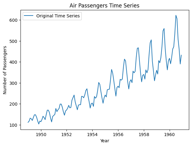
Step 2: Dataset loading and visualization

Next, we load a time-series dataset (e.g., US Airline Passengers) from Kaggle. We then visualize the original data to identify any patterns.

You can download the dataset from here.

data = pd.read_csv('AirPassengers.csv')
data['Month'] = pd.to_datetime(data['Month'], format='%Y-%m')
data.set_index('Month', inplace=True)

# Plot the original time series data
plt.figure(figsize=(7, 5))
plt.plot(data, label='Original Time Series')
plt.title('Air Passengers Time Series')
plt.xlabel('Year')
plt.ylabel('Number of Passengers')
plt.legend()
plt.show()

Output

Step 3: Data decomposition

Decompose the time series into trend, seasonal and residual components. We'll use a multiplicative model since the seasonal pattern is constant over different levels of the series.

# Decompose the time series into trend, seasonal and residual components
result = seasonal_decompose(
    data, model='multiplicative', extrapolate_trend='freq')
result.plot()
plt.suptitle('Seasonal Decomposition of Air Passengers Time Series')
plt.tight_layout()
plt.show()

Output

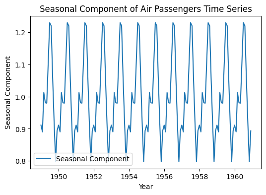
Step 4: Visualizing the seasonality

Now we will visualize the only seasonal component by extracting it from the decomposition results.

# Plot the seasonal component
plt.figure(figsize=(6, 4))
plt.plot(result.seasonal, label='Seasonal Component')
plt.title('Seasonal Component of Air Passengers Time Series')
plt.xlabel('Year')
plt.ylabel('Seasonal Component')
plt.legend()
plt.show()

Output

Step 5: Removing seasonality from the data

To use a time-series data for various purposes including model training it is required to have a seasonality free time-series data.

Equation:

d(t) = y(t) - y(t - m)

Where:

• d (t) is the differenced data point at time t.
• y (t) is the value of the series at time t.
• y (t - m) is the value of the data point at the previous season.
• m is the length of one season (in this case, m = 12 as we have yearly seasonality).

This equation represents seasonal differencing, used to remove the seasonal component from the data.

Here we will visualize how organized it will look after removing the seasonality.

# Plotting the original data and original data without the seasonal component
plt.figure(figsize=(7, 4))

# Plot the original time series data
plt.plot(data, label='Original Time Series', color='blue')
data_without_seasonal = data['#Passengers'] / result.seasonal

# Plot the original data without the seasonal component
plt.plot(data_without_seasonal,
         label='Original Data without Seasonal Component', color='green')
plt.title('Air Passengers Time Series with and without Seasonal Component')
plt.xlabel('Year')
plt.ylabel('Number of Passengers')
plt.legend()
plt.show()

Output

From the plot we can see that after removing seasonality the time-series data became very organized.

Step 6: Applying the Augmented Dickey-Fuller (ADF) Test

After removing seasonality, it is important to verify whether the time series has become stationary. The Augmented Dickey-Fuller (ADF) test is commonly used for this purpose, as it checks the null hypothesis that the series contains a unit root, indicating non-stationarity.

Here’s how we can perform the ADF test:

from statsmodels.tsa.stattools import adfuller

adf_result = adfuller(data_without_seasonal)

print('ADF Statistic:', adf_result[0])
print('p-value:', adf_result[1])

#Interpreting the results
if
    adf_result[1] < 0.05 : print("The data is stationary (p-value < 0.05).")
else:
    print("The data is not stationary (p-value >= 0.05).")

Output

ADF Statistic: 1.1415289777074211
p-value: 0.9955559262862962
The data is not stationary (p-value >= 0.05).

Even after removing seasonality, a p-value greater than 0.05 in the ADF test indicates the data is still non-stationary, likely due to an underlying trend. Additional differencing may be required to remove the trend and achieve stationarity.

Therefore, the data is not yet ready for model training without further transformation. First differencing or additional decomposition may be required to fully prepare the data for time series forecasting.

Step 7: Differencing the Data

Differencing is applied to remove remaining trends in the data and reassess stationarity using the ADF test.

data_diff = data_without_seasonal.diff().dropna()
adf_result = adfuller(data_diff)
print('ADF Statistic:', adf_result[0])
print('p-value:', adf_result[1])

Output

ADF Statistic: -2.9058136872756286
p-value: 0.04467610954112502

After seasonal adjustment, the ADF test initially indicated non-stationarity (p-value = 0.9955), suggesting a remaining trend. Applying differencing reduced the p-value to 0.0447, confirming the data is now stationary and suitable for forecasting.

Visualizing after differencing the data:

plt.figure(figsize=(7, 4))

plt.plot(data, label='Original Time Series', color='blue')

plt.plot(data_diff, label='Differenced Data', color='orange')

plt.title('Original Time Series vs Differenced Data')
plt.xlabel('Year')
plt.ylabel('Number of Passengers')
plt.legend()
plt.show()

Output