Semi supervised classification is a technique in data mining that uses both labeled and unlabeled data to build a classification model. Usually, only a small portion of the dataset has labels, while the remaining data is unlabeled. The model learns patterns from both types of data to improve classification performance.
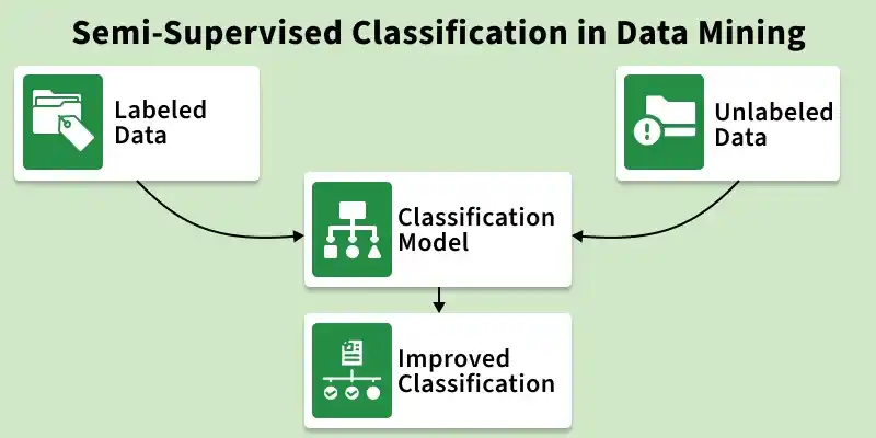
- Uses both labeled and unlabeled data.
- Only a small portion of data is labeled.
- Most data remains unlabeled.
- Useful when labeling data is difficult or costly.
- Combines supervised and unsupervised learning
Working
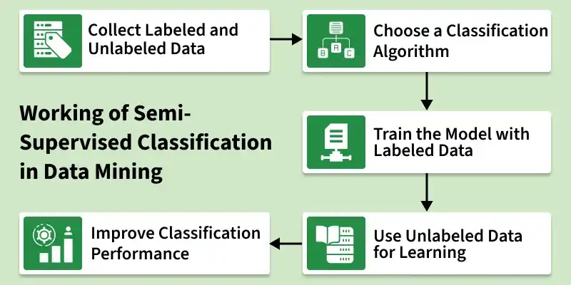
The working of semi supervised classification in data mining can be explained in the following steps:
1. Collect Labeled and Unlabeled Data: Gather a dataset that contains a small amount of labeled data and a large amount of unlabeled data.
Example: A few images of animals with labels and many images without labels.
2. Choose a Classification Algorithm: Select a suitable classification algorithm that can work with both labeled and unlabeled data.
3. Train the Model with Labeled Data: The model first learns patterns and relationships using the available labeled data.
4. Use Unlabeled Data for Learning: The model then uses the unlabeled data to discover additional patterns and improve its understanding.
5. Improve Classification Performance: By combining both types of data, the model becomes better at classifying new or unseen data.
Implementation
Step 1: Import Required Libraries
Import the necessary Python libraries for data handling, machine learning and evaluation.
import numpy as np
import pandas as pd

import matplotlib.pyplot as plt
import seaborn as sns

from sklearn.datasets import load_iris
from sklearn.model_selection import train_test_split
from sklearn.semi_supervised import LabelPropagation
from sklearn.metrics import accuracy_score, confusion_matrix
Step 2: Load the Dataset
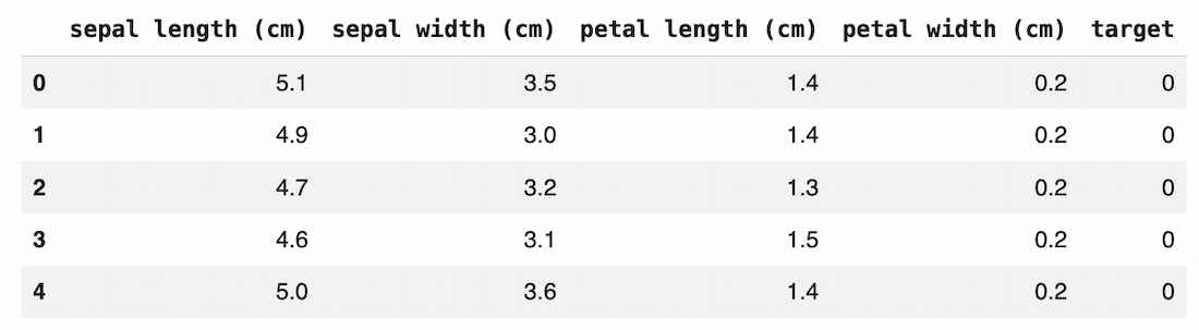
- The Iris dataset is loaded from sklearn.
- It contains 150 samples and 3 flower classes.
- Features represent measurements of petals and sepals.
data = load_iris()

X = data.data
y = data.target

df = pd.DataFrame(X, columns=data.feature_names)
df["target"] = y

df.head()
Output:
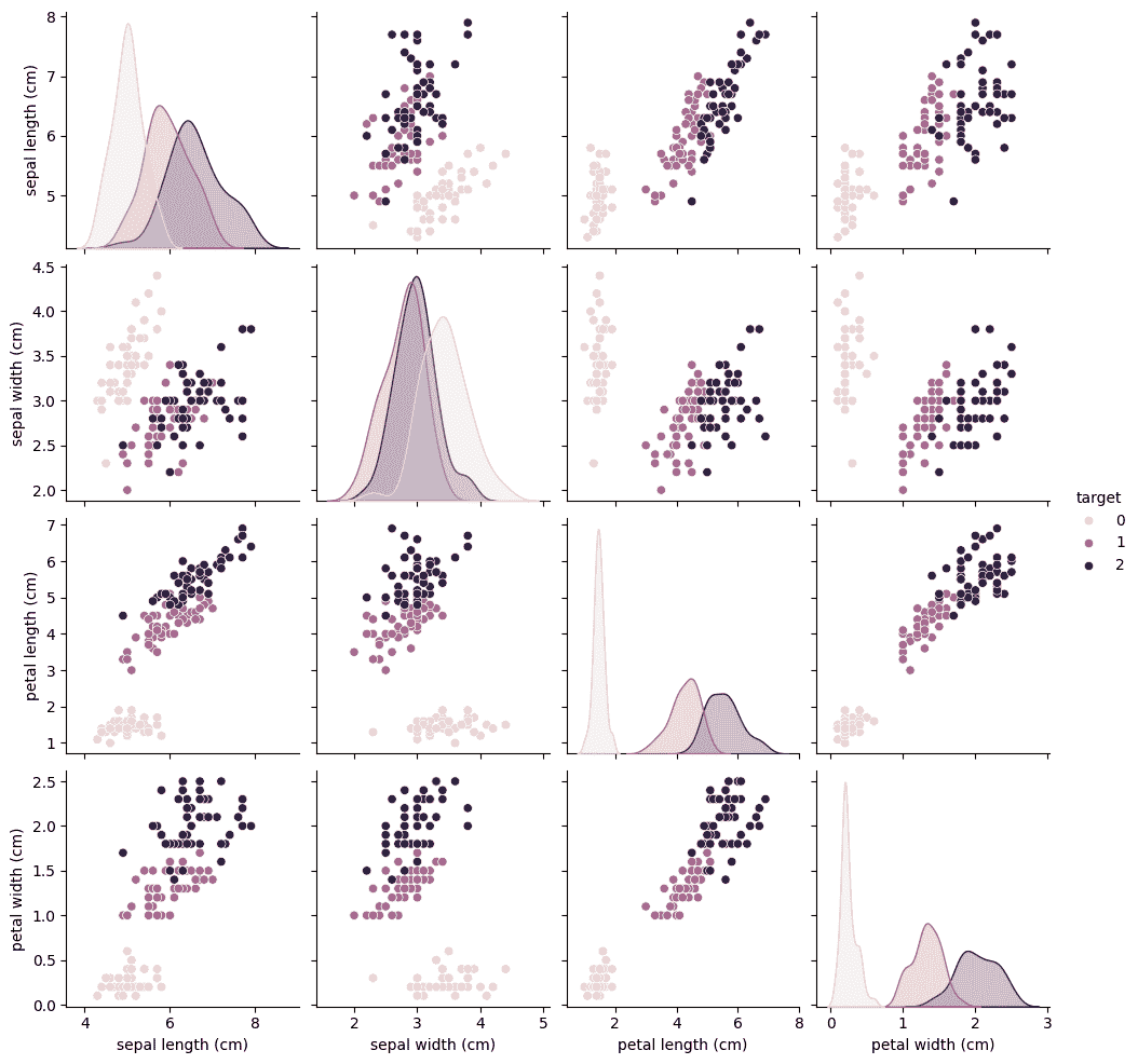
Step 3: Visualize the Dataset
This visualization shows relationships between features.
- Each color represents a different class.
- It helps understand how the classes are distributed.
- Good separation between classes makes classification easier.
sns.pairplot(df, hue="target")
plt.show()
Output:
Step 4: Split the Dataset
- 70% of data is used for training.
- 30% of data is used for testing.
- The model learns from training data and is evaluated on test data.
X_train, X_test, y_train, y_test = train_test_split(
    X, y, test_size=0.3, random_state=42
)
Step 5: Create Unlabeled Data
Semi supervised learning assumes that most data is unlabeled.
- Some training labels are removed.
- -1 represents unlabeled samples.
- The model will try to infer these labels during training.
y_train_semi = y_train.copy()

rng = np.random.RandomState(42)
random_unlabeled = rng.rand(len(y_train_semi)) < 0.7

y_train_semi[random_unlabeled] = -1
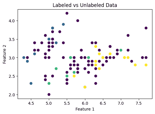
Step 6: Visualize Labeled vs Unlabeled Data
This plot shows the distribution of labeled and unlabeled samples.
- Colored points represent labeled data.
- Dark points represent unlabeled data.
- This demonstrates the semi-supervised setting.
plt.figure(figsize=(6,4))

plt.scatter(X_train[:,0], X_train[:,1], c=y_train_semi, cmap="viridis")

plt.title("Labeled vs Unlabeled Data")
plt.xlabel("Feature 1")
plt.ylabel("Feature 2")

plt.show()
Output:
Step 7: Train the Semi Supervised Model
The model learns patterns using:
- Available labeled data
- Structure of unlabeled data
model = LabelPropagation()

model.fit(X_train, y_train_semi)
Step 8: Predict the Test Data
The trained model predicts the class of unseen samples.
predictions = model.predict(X_test)
Step 9: Evaluate Model Accuracy
- Accuracy measures how many predictions are correct.
- Higher accuracy means the classification model performs better.
accuracy = accuracy_score(y_test, predictions)

print("Accuracy:", accuracy)
Output:
Accuracy: 1.0
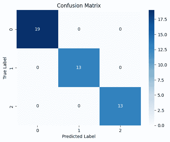
Step 10: Confusion Matrix Visualization
The confusion matrix shows:
- Correct predictions along the diagonal
- Misclassifications in other cells
cm = confusion_matrix(y_test, predictions)

sns.heatmap(cm, annot=True, cmap="Blues")

plt.title("Confusion Matrix")
plt.xlabel("Predicted Label")
plt.ylabel("True Label")

plt.show()
Output:
Download full code from here
Applications
- Used in audio data to improve speech recognition systems.
- Since billions of web pages exist, labeling them manually is not practical. It helps automatically classify and organize web content.
- Uses a few labeled texts and many unlabeled ones to classify documents into categories.
Advantages
- Semi supervised classification is relatively simple to understand and implement because it combines ideas from supervised and unsupervised learning.
- Requires only a small amount of labeled data, which reduces the effort and cost involved in manually labeling large datasets.
- Algorithm can still learn useful patterns by using a large amount of unlabeled data along with the available labeled samples.
Disadvantages
- Results of the algorithm may change across different iterations because the model continuously updates labels during training.
- May not effectively capture complex relationships present in large network or graph based datasets.
- Accuracy may not always be high, especially when the unlabeled data contains noise or misleading patterns.
