Spline regression is a flexible method used in statistics and machine learning to fit a smooth curve to data points by dividing the independent variable (usually time or another continuous variable) into segments and fitting separate polynomial functions to each segment. This approach avoids the limitations of linear models by allowing the curve to bend at specified points, called knots, thereby capturing nonlinear relationships between variables more accurately.
In this article, we will explore spline regression in R Programming Language covering its concepts, implementation using different packages, and interpretation of results.
Types of Splines
Now we will discuss the different types of Splines.
- Piecewise Polynomial Splines: These splines fit different polynomials in different intervals defined by knots.
- Natural Splines: These splines impose additional constraints at the boundary knots to ensure smoothness at the edges of the data range.
- Cubic Splines: These are a type of piecewise polynomial spline where each segment is a cubic polynomial. They ensure continuity in the first and second derivatives at the knots.
Now we will discuss step by step to implement Spline Regression in R Programming Language.
Step 1. Installing and Loading Required Packages
To perform spline regression in R, you'll need the `splines` package. Additionally, for accessing example datasets, we install and load the `Ecdat` package.
install.packages('splines')
install.packages('Ecdat')

library(splines)
library(Ecdat)
Step 2. Preparing Data for Spline Regression
To prepare for spline regression using the Clothing dataset from the Ecdat package in R, we first load the dataset and then visualize it to understand its structure and characteristics. Loading the Clothing dataset allows us to inspect its variables and relationships visually, which is crucial for preparing and understanding the data before fitting spline regression models.
data(Clothing)
head(Clothing)
Output:
   tsales     sales margin nown  nfull  npart   naux hoursw  hourspw      inv1     inv2
1  750000  4411.765     41    1 1.0000 1.0000 1.5357     76 16.75596  17166.67 27177.04
2 1926395  4280.878     39    2 2.0000 3.0000 1.5357    192 22.49376  17166.67 27177.04
3 1250000  4166.667     40    1 2.0000 2.2222 1.4091    114 17.19120 292857.20 71570.55
4  694227  2670.104     40    1 1.0000 1.2833 1.3673    100 21.50260  22207.04 15000.00
5  750000 15000.000     44    2 1.9556 1.2833 1.3673    104 15.74279  22207.04 10000.00
6  400000  4444.444     41    2 1.9556 1.2833 1.3673     72 10.89885  22207.04 22859.85
  ssize start
1   170    41
2   450    39
3   300    40
4   260    40
5    50    44
6    90    41
Step 3. Building Spline Regression Models with Choosing the Number and Location of Knots
Next, we proceed to build a spline regression model using the lm function in R, incorporating B-spline basis functions generated by the bs function from the splines package. This approach allows us to fit a regression model that can effectively capture nonlinear relationships present in the data.
model <- lm(tsales ~ bs(inv2, knots = c(12000, 60000, 150000)), data = Clothing)
summary(model)
Output:
Call:
lm(formula = tsales ~ bs(inv2, knots = c(12000, 60000, 150000)),
    data = Clothing)

Residuals:
    Min      1Q  Median      3Q     Max
-921708 -329164 -125551  223018 3598276

Coefficients:
                                           Estimate Std. Error t value Pr(>|t|)
(Intercept)                                  419589     136370   3.077 0.002238 **
bs(inv2, knots = c(12000, 60000, 150000))1   712180     213810   3.331 0.000948 ***
bs(inv2, knots = c(12000, 60000, 150000))2    63428     140939   0.450 0.652929
bs(inv2, knots = c(12000, 60000, 150000))3   847253     269728   3.141 0.001810 **
bs(inv2, knots = c(12000, 60000, 150000))4  1308842     707178   1.851 0.064949 .
bs(inv2, knots = c(12000, 60000, 150000))5   -14067     996832  -0.014 0.988748
bs(inv2, knots = c(12000, 60000, 150000))6  1345263     419450   3.207 0.001450 **
---
Signif. codes:  0 ‘***’ 0.001 ‘**’ 0.01 ‘*’ 0.05 ‘.’ 0.1 ‘ ’ 1

Residual standard error: 562100 on 393 degrees of freedom
Multiple R-squared:  0.08582,    Adjusted R-squared:  0.07186
F-statistic: 6.149 on 6 and 393 DF,  p-value: 3.54e-06
Step 4. Visualizing Spline Regression Results
Visualize the fitted spline regression line along with confidence intervals to understand how well the model fits the data.
inv2lims <- range(Clothing$inv2)
inv2.grid <- seq(from = inv2lims[1], to = inv2lims[2])
pred <- predict(model, newdata = list(inv2 = inv2.grid), se = TRUE)

plot(Clothing$inv2, Clothing$tsales, main = "Regression Spline Plot",
     xlab = "Inventory", ylab = "Total Sales")
lines(inv2.grid, pred$fit, col = 'green', lwd = 3)
lines(inv2.grid, pred$fit + 4 * pred$se.fit, lty = "dashed", lwd = 4, col = 'red')
lines(inv2.grid, pred$fit - 4 * pred$se.fit, lty = "dashed", lwd = 4, col = 'red')
segments(12000, 0, x1 - 12000, y1 - 5000000, col = 'black')
segments(60000, 0, x1 - 60000, y1 - 5000000, col = 'black')
segments(150000, 0, x1 - 150000, y1 - 5000000, col = 'black')
Output:

Step 5: Comparing Spline Regression with Linear Regression
Contrasting spline regression with linear regression underscores the advantages of splines in capturing nonlinear relationships in data. Unlike linear regression, which assumes a constant relationship between variables, spline regression allows for more flexible modeling by fitting piecewise polynomials that can adapt to changing patterns in the data.
linear_model <- lm(tsales ~ inv2, data = Clothing)
summary(linear_model)

plot(Clothing$inv2, Clothing$tsales,main = "Comparison of Linear and Spline Regression",
     xlab = "Inventory", ylab = "Total Sales")
lines(inv2.grid, predict(linear_model, newdata = list(inv2 = inv2.grid)), col = 'blue')
lines(inv2.grid, pred$fit, col = 'red')
legend("topleft", legend = c("Linear Regression", "Spline Regression"),
       col = c("blue", "red"), lty = 1)
Output:
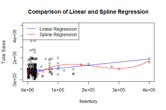
This flexibility enables splines to better capture complex and nonlinear relationships, offering improved accuracy in modeling real-world phenomena where relationships may vary across different ranges or segments of the predictor variable. By accommodating such variations, splines mitigate the limitations of linear models, making them suitable for datasets with intricate and nonlinear structures.
Advanced Techniques and Options for Spline Regression in R
Explore advanced techniques in spline regression such as using different types of splines and generalized additive models (GAMs) for more complex data patterns.
# Smoothing spline
smooth_fit <- smooth.spline(Clothing$inv2, Clothing$tsales)
lines(smooth_fit, col = "green")

# GAM
library(mgcv)
gam_fit <- gam(tsales ~ s(inv2), data = Clothing)
lines(inv2.grid, predict(gam_fit, newdata = list(inv2 = inv2.grid)), col = "purple")

legend("topright", legend = c("Smoothing Spline", "GAM"),
       col = c("green", "purple"), lty = 1)
Output:

Spline regression is highly effective in modeling seasonal sales trends, where sales data exhibit complex patterns over time.
- For instance, a retail business might experience fluctuating sales due to holidays, promotions, and seasonal changes.
- By applying spline regression, analysts can segment the sales data into different periods and fit separate polynomials for each segment.
- This approach helps in capturing intricate seasonal variations, providing better insights for inventory management, marketing strategies, and forecasting future sales trends.
Conclusion
Spline regression is a versatile and powerful tool for modeling nonlinear relationships in data. By understanding how to implement and evaluate spline regression in R, you can enhance your data analysis and predictive modeling capabilities. Whether you're handling nonlinear trends or fitting piecewise polynomials, spline regression offers a robust solution for many statistical challenges.
