YOLO : You Only Look Once - Real Time Object Detection

YOLO (You Only Look Once) is a deep learning-based object detection algorithm that identifies and localizes objects within an image in a single pass through the network. By treating object detection as a unified task, YOLO provides a fast and efficient solution for detecting multiple objects in real time.

• Predicts object classes and bounding box locations simultaneously.
• Delivers high-speed detection while maintaining good accuracy.

YOLO Architecture

1. Input Preprocessing

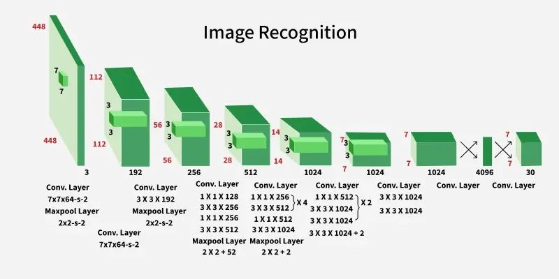
The model accepts an input image and resizes it to 448 × 448 pixels, preserving the aspect ratio through padding. This provides uniform input dimensions for efficient processing by the network.

2. Backbone Convolutional Neural Network (CNN)

After preprocessing the image is passed through a deep CNN architecture designed for object detection:

• The model consists of 24 convolutional layers and 4 max-pooling layers.
• These layers help in extracting hierarchical spatial features from the image.

3. Convolutional Layers

The architecture combines:

• 1 × 1 convolutions for channel reduction and computational efficiency.
• 3 × 3 convolutions for capturing spatial features.

This design pattern i.e 1×1 followed by 3×3 improves computational efficiency while maintaining expressive power.

4. Fully Connected Layers

Following the convolutional layers, the architecture has 2 fully connected layers. The final fully connected layer produces an output of shape (1, 1470).

5. Cuboidal Prediction Output

The output vector of size 1470 is reshaped to (7, 7, 30). Here, 7×7 represents the grid cells, and 30 represents the prediction vector for each cell.

30 = (2 \text{ bounding boxes} \times 5) + (20 \text{ class probabilities})

6. Activation Functions

The architecture predominantly uses Leaky ReLU as its activation function. The Leaky ReLU is defined as:

f(x) = \begin{cases} x, & \text{if } x > 0 \\ 0.01x, & \text{if } x \leq 0 \end{cases}

This activation allows a small gradient when the unit is not active, preventing dead neurons.

7. Output Layer Activation

The last layer uses a linear activation function, suitable for making raw predictions like bounding box coordinates and confidence scores.

8. Regularization Techniques

• Batch Normalization improves training stability and convergence.
• Dropout reduces overfitting and enhances generalization.

This version removes repetitive explanations while preserving all important architectural components.

Training Process

1. Dataset and Training

YOLO is trained on the ImageNet-1000 dataset for feature learning before being adapted for object detection. A lightweight variant, Fast YOLO, uses fewer convolutional layers and filters, resulting in faster inference.

2. YOLO Loss Function

YOLO uses a sum-squared error loss function to optimize object localization and classification simultaneously.

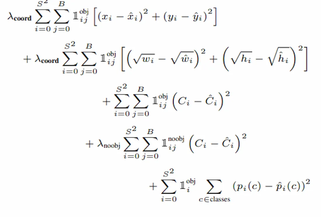
Where:

• l_{i}^{obj} denotes if object is present in cell i. 
• l_{ij}^{obj} denotes j_{th} bounding box responsible for prediction of object in the cell i. 
• \lambda_{coord} and \lambda_{noobj} are balancing parameters for the loss function.

3. Localization Error

Localization loss measures the error between the predicted bounding boxes and the ground-truth object locations.

• The first term calculates the deviation in the predicted bounding box coordinates.
• The second term evaluates errors in the predicted width and height, giving greater importance to small bounding boxes by using their square roots.

4. Classification Loss

Classification loss measures the model's ability to correctly identify objects and predict their classes. It consists of three components:

• Error between the predicted confidence score and the actual object presence for each bounding box.
• Error from grid cells that do not contain any object, scaled using a regularization parameter to prevent these cells from dominating the loss.
• Error between the predicted class probabilities and the ground-truth object classes.

This formulation helps YOLO balance object localization, confidence prediction, and classification during training.

Object Detection Using YOLO

1. Grid-Based Detection

YOLO divides the input image into an S × S grid, where each grid cell is responsible for detecting objects whose center lies within that cell.

• Each grid cell predicts multiple bounding boxes and their confidence scores.
• The confidence score indicates the likelihood of an object being present and the accuracy of the predicted bounding box.

2. Bounding Box Prediction

Each predicted bounding box contains five values:

• (x, y): Coordinates of the bounding box center relative to the grid cell.
• (w, h): Width and height of the bounding box.
• Confidence Score: Indicates the presence of an object and the quality of localization.

The confidence score is defined as:

\kern 6pc P_{r}\left( \text{Object} \right) * \text{IOU}_{\text{pred}}^{\text{truth}}

where IoU (Intersection over Union) measures the overlap between the predicted bounding box and the ground-truth box.

3. Class Probability Prediction

In addition to bounding boxes, each grid cell predicts conditional class probabilities for the object classes.

• The probabilities are represented as Pr(Classi∣Object)Pr(Class_i \mid Object)Pr(Classi​∣Object).
• Predictions are encoded in a tensor of size S × S × (5B + C), where B is the number of bounding boxes and C is the number of classes.

4. Final Detection Output

The conditional class probabilities are multiplied by the corresponding confidence scores to obtain class-specific confidence values for each bounding box.

• Multiple overlapping predictions are filtered using Non-Maximum Suppression (NMS).
• The remaining boxes form the final object detection results.

Importance

• Real-Time Detection: Processes images in a single forward pass, enabling fast object detection.
• End-to-End Learning: Performs object localization and classification within a unified network.
• Global Image Understanding: Considers the entire image during prediction, reducing background errors.
• High Efficiency: Requires fewer computational resources compared to multi-stage detection methods.