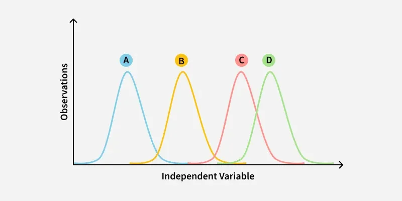
ANOVA (Analysis of Variance) is a statistical technique used to determine whether there is a significant difference between the means of three or more groups. It tests the null hypothesis that all group means are equal.
ANOVA works by comparing:
- Between-group variation – differences among the group means.
- Within-group variation – natural differences among observations within the same group.
Using the F-statistic, ANOVA evaluates whether the variation between groups is larger than the variation within groups. If it is, ANOVA indicates that at least one group mean is significantly different; otherwise, the observed differences are likely due to chance.
For example:
Compare test scores of students taught with 3 methods (Traditional, Online, Hybrid). ANOVA is used to determine if at least one teaching method yields significantly different average scores.
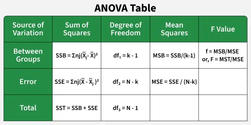
ANOVA Formula
The ANOVA formula is made up of numerous parts. The best way to tackle an ANOVA test problem is to organize the formulae inside an ANOVA table.
Here's a general structure of an ANOVA table:
where,
- F = ANOVA Coefficient
- MSB = Mean of the total of squares between groupings
- MSW = Mean total of squares within groupings
- MSE = Mean sum of squares due to error
- SST = total Sum of squares
- p = Total number of populations
- n = The total number of samples in a population
- SSW = Sum of squares within the groups
- SSB = Sum of squares between the groups
- SSE = Sum of squares due to error
- s = Standard deviation of the samples
- N = Total number of observations
Assumptions of ANOVA
These must be validated before analysis:
- Independence: Observations are randomly sampled, and groups are independent.
- Normality: Residuals (errors) are approximately normally distributed (checked via Q-Q plots or Shapiro-Wilk test).
- Homoscedasticity: Equal variances across groups (verified using Levene’s or Bartlett’s test).
ANOVA is robust to minor violations of normality and homoscedasticity with balanced sample sizes.
Calculating ANOVA
Compare plant growth under 3 fertilizers (A, B, and C):
- Fertilizer A: [10, 11, 12]
- Fertilizer B: [7, 8, 9]
- Fertilizer C: [4, 5, 6]
1. State Hypothesis
- Null Hypothesis (H0): μA = μB = μC
- Alternative Hypothesis (Ha): At least one μ differs.
2. Calculate Group means and Grand mean.
- Group Means:
\bar X_A, \bar X_B, and \bar X_C - Grand Mean:
\overline{X}_{\text{grand}}
3. Compute Sum of Squares (SS):
SSB (Sum of Squares Between Groups): Accounts for variation due to the treatment or independent variable.
SSB = \sum n_i(\bar{X}_i - \bar{X}_{\text{grand}})^2
SSE (Sum of Squares Error or Within Groups): Accounts for variation within groups (random error or residuals).SSE = \sum ({x}_i - \bar{X})^2 SST (Total Sum of Squares): Accounts for total variation from overall mean.
SST = SSB + SSW
SSB = 3(11 − 8) + 3(8 − 8) + 3(5 − 8) = 3(9) + 3(0) + 3(9) = 54
SSE:
- Fertilizer A: (10 − 11) + (11 − 11) + (12 − 11) = 1 + 0 + 1 = 2
- Fertilizer B: (7 − 8) + (8 − 8) + (9 − = 1 + 0 + 1 = 2
- Fertilizer C: (4 − 5) + (5 − 5) + (6 − 5) = 1 + 0 + 1 = 2
SSW = 2 + 2 + 2 = 6
SST = 54 + 6 = 60
4. Calculate Degrees of Freedom (df):
df1 (Between Groups) = k - 1, where k is number of groups.
df2 (Within Groups) = N - k, where N is the total observations.
df3 (Total) = N - 1.
- df1 = 3 - 1 = 2
- df2 = 9 - 3 = 6
- df3 = 9 - 1 = 8
5. Calculate Mean Squares (MS):
MSB (Mean Square Between Groups) = SSB / df1.
MSE (Mean Square Error) = SSE / df2.
MSB = \frac{SSB}{df1} = \frac{54}{2} = 27 MSW = \frac{SSW}{df2} = \frac{6}{6} = 1
6. F-statistic:
The F-statistic is calculated as the ratio of MSB to MSE:
F = \frac{MSB}{MSE}
F = \frac{27}{1} = 27
7. P-value:
The p-value is used to decide whether differences among groups are statistically significant. When the p-value is smaller than the significance level (α), the null hypothesis is rejected.
If F > Fcritical → p < 0.05 : Null Hypothesis Rejected
Use the F-distribution table or software with the following: Numerator df1 = 2, Denominator df2 = 6, α = 0.05
Critical F-value, Fcritical: 5.14 (From F-distribution table)
F > Fcritical: 27 > 5.14 → p < 0.05; Reject null hypothesis
Types of ANOVA
ANOVA is mainly classified into two types based on the number of independent variables (factors) being studied.
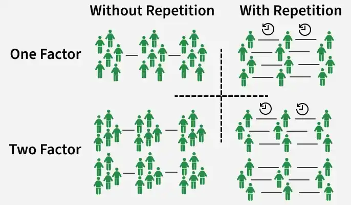
1. One-Way ANOVA (or One-Factor)
One-Way ANOVA is used to compare the means of three or more groups when there is only one independent variable. It helps determine whether the differences among the group means are statistically significant.
Example: Comparing the average test scores of students taught using three different teaching methods.
2. Two-Way ANOVA (or Two-Factor)
Two-Way ANOVA is used when there are two independent variables. It evaluates the effect of each factor on the dependent variable and also determines whether the two factors interact with each other.
Example: Studying how students' test scores are affected by both the teaching method and the number of study hours.
Solved Examples
Example 1: Three different kinds of food are tested on three groups of rats for 5 weeks. The objective is to check the difference in mean weight (in grams) of the rats per week. Apply one-way ANOVA using a 0.05 significance level to the following data:
| Food I | Food II | Food III |
|---|---|---|
| 8 | 4 | 11 |
| 12 | 5 | 8 |
| 19 | 4 | 7 |
| 8 | 6 | 13 |
| 6 | 9 | 7 |
| 11 | 7 | 9 |
Solution:
H0: μ1= μ2=μ3
H1: The means are not equalSince, X̄1 = 5, X̄2 = 9, X̄3 = 10
Total mean = X̄ = 8
- SSB = 6(5 - 8)2 + 6(9 - 8)2 + 6(10 - 8)2 = 84
- SSE = 68
- MSB = SSB/df1 = 42
- MSE = SSE/df2 = 4.53
- f = MSB/MSE = 42/4.53 = 9.33
Since f > F, the null hypothesis stands rejected.
Example 2: Calculate the ANOVA coefficient for the following data:
| Plant | Number | Average span | s |
|---|---|---|---|
| Hibiscus | 5 | 12 | 2 |
| Marigold | 5 | 16 | 1 |
| Rose | 5 | 20 | 4 |
Solution:
Plant n x s s2 Hibiscus 5 12 2 4 Marigold 5 16 1 1 Rose 5 20 4 16 p = 3
n = 5
N = 15
x̄ = 16SST = Σn(x−x̄)2
- SST= 5(12 − 16)2 + 5(16 − 16)2 + 11(20 − 16)2 = 160
- MST = SST/p-1 = 160/3-1 = 80
- SSE = ∑ (n−1) = 4 (4 + 1) + 4(16) = 84
- MSE = 7
- F = MST/MSE = 80/7
- F = 11.429
Example 3: The following data show the number of worms quarantined from the GI areas of four groups of muskrats in a carbon tetrachloride anthelmintic study. Conduct a two-way ANOVA test.
| I | II | III | IV |
|---|---|---|---|
| 338 | 412 | 124 | 389 |
| 324 | 387 | 353 | 432 |
| 268 | 400 | 469 | 255 |
| 147 | 233 | 222 | 133 |
| 309 | 212 | 111 | 265 |
Solution:
Source of Variation Sum of Squares Degrees of Freedom Mean Square Between the groups 62111.6 8 9078.067 Within the groups 98787.8 16 4567.89 Total 167771.4 24 Since F = MST / MSE
= 9.4062 / 3.66
F = 2.57
Example 4: Enlist the results in APA format after performing ANOVA on the following data set:
Solution:
- Variance of first set = (10.45)2 = 109.2
- Variance of second set = (12.76)2 = 162.82
- Variance of third set = (11.47)2 = 131.56
MSerror = {109.2 + 162.82 + 131.56} / {3}
= 134.53MSbetween = (17.62)(30) = 528.75
F = MSbetween / MSerror
= 528.75 / 134.53
F = 4.86APA writeup: F(2, 87)=3.93, p >=0.01, η2=0.08.
Practice Problem
Question 1. Method A = {80, 85, 90, 87}, Method B = {75, 78, 72, 74}, and Method C = {88, 85, 90, 92} are given. State the null and alternative hypotheses for performing a One-Way ANOVA test.
Question 2. Calculate the F-statistic for the given data using One-Way ANOVA. Group 1 = {5, 6, 7, 8}, Group 2 = {4, 5, 6, 5}, and Group 3 = {7, 7, 6, 8}.
Question 3. Interpret the significance of the p-value for the interaction effect in a Two-Way ANOVA, where the p-value for the interaction effect is 0.02 and the significance level (α) is 0.05.
Question 4. Group A = {10, 12, 14, 13}, Group B = {15, 17, 16, 18}, and Group C = {20, 22, 21, 23} are given. Interpret the p-value of the ANOVA test and explain whether the null hypothesis is rejected, where F-statistic = 4.86 and p-value = 0.01.
Answer:-
- Null Hypothesis (H₀): μ₁ = μ₂ = μ₃ (The means of all groups are equal). Alternative Hypothesis (H₁): At least one mean is different.
- F-statistic = 4.58.
- If the p-value (0.02) is less than the significance level (0.05), reject the null hypothesis and conclude that there is a significant interaction effect.
- Since the p-value (0.01) is less than 0.05 and the F-statistic is significant, we reject the null hypothesis, indicating a significant difference between the group means.
