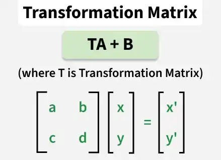
A transformation matrix is a square matrix that represents a linear transformation of vectors. It is used to perform operations such as rotation, scaling, reflection, and shearing by multiplying the matrix with a vector. The matrix defines how points or vectors are transformed while preserving the linear properties of the space.
Example: Imagine a 2D coordinate system with the usual direction vectors i (for the x-axis) and j (for the y-axis).
Let’s say you have a vector: v = (x, y)
Now, you apply a transformation matrix T to this vector. It gives a new vector: w = (x′, y).
The transformation matrix T changes the direction or size of the vector and gives you a new version of it.
Types of Transformation Matrix
Transformation matrices are classified based on the geometric transformation they perform. Some common types of transformation matrices include:
1. Translation Matrix
A translation matrix is used to shift objects in a coordinate system.
Example: Let's consider a point P(2, 3) and apply a translation of (4, 1) units.
Solution:
Given point P = (2, 3) and translation vector T = (4, -1), the translation matrix is:
\begin{pmatrix} 1 & 0 & 4\\ 0 & 1 & -1\\ 0 & 0 & 1\\ \end{pmatrix} Applying the translation matrix to point P:
\begin{pmatrix} 1 & 0 & 4\\ 0 & 1 & -1\\ 0 & 0 & 1\\ \end{pmatrix} \begin{pmatrix} 2\\ 3\\ 1\\ \end{pmatrix} =\begin{pmatrix} 6\\ 2\\ 1\\ \end{pmatrix} Therefore, after the translation, point P(2, 3) is moved to P'(6, 2).
2. Rotation Matrix
A rotation matrix is used to rotate objects in a coordinate system.
Example: Let's rotate a point Q(1, 1) by 90 degrees counterclockwise.
Solution:
Given point Q = (1, 1) and rotation angle θ = 90 degrees, the rotation matrix is:
R =
\begin{pmatrix} 0 & -1\\ 1 & 0\\ \end{pmatrix} Applying the rotation matrix to point Q:
\begin{pmatrix} 0 & -1\\ 1 & 0\\ \end{pmatrix} \begin{pmatrix} 1\\ 1\\ \end{pmatrix} =\begin{pmatrix} -1 \\ 1\\ \end{pmatrix} After the rotation, point Q(1, 1) is rotated to Q'(-1, 1).
3. Scaling Matrix
A scaling matrix is used to resize objects in a coordinate system.
Example: Let's scale a rectangle with vertices A(1, 1), B(1, 3), C(3, 3), and D(3, 1) by a factor of 2 in the x-direction and 3 in the y-direction.
Solution:
Given rectangle ABCD and scaling factors sx = 2, sy = 3, the scaling matrix is:
S =
\begin{pmatrix} 2 & 0\\ 0 & 3\\ \end{pmatrix} Applying the scaling matrix to the vertices of the rectangle:
A'(2, 3), B'(2, 9), C'(6, 9), D'(6, 3)
4. Combined Matrix
A combined matrix applies multiple transformations in sequence.
Example: Let's translate point P(1, 2) to (3, 4) and then rotate it 45 degrees counterclockwise.
Solution:
Given point P = (1, 2), translation vector T = (3, 4), rotation angle θ = 45 degrees, the combined matrix is:
C = R⋅T
Applying the combined matrix to point P:
First, translate by T:
T =
\begin{pmatrix} 1 & 0 & 3\\ 0 & 1 & 4\\ 0 & 0 & 1\\ \end{pmatrix} P′ = T⋅P =
\begin{pmatrix} 4\\ 6\\ 1\\ \end{pmatrix} Then, rotate by R:
R =
\begin{pmatrix} cos(45) & −sin(45)\\ sin(45) & cos(45)\\ \end{pmatrix} P′′ = R⋅P′ =
\begin{pmatrix} -1\\ 5\\ \end{pmatrix}
5. Reflection Matrix
A reflection matrix is used to mirror objects across a line or plane.
Example: Let's reflect a point Q(2, 3) across the x-axis.
Solution:
Given point Q = (2, 3), the reflection matrix about the x-axis is:
Rx =
\begin{pmatrix} 1 & 0\\ 0 & -1\\ \end{pmatrix} Applying the reflection matrix to point Q:
Rx⋅Q =
\begin{pmatrix} 2\\ -3\\ \end{pmatrix} After reflection, point Q(2, 3) is mirrored to Q'(2, -3).
6. Shear Matrix
A shear matrix is used to skew objects in a coordinate system.
Example: Let's shear a rectangle with vertices A(1, 1), B(1, 3), C(3, 3), D(3, 1) in the x-direction by a factor of 2.
Solution:
Given rectangle ABCD and shear factor kx = 2, the shear matrix is:
Hx =
\begin{pmatrix} 1 & 2\\ 0 & 1\\ \end{pmatrix} Applying the shear matrix to the vertices of the rectangle:
A'(3, 1), B'(7, 3), C'(9, 3), D'(5, 1)
7. Affine Transformation Matrix
An affine transformation matrix combines linear transformations with translations. Let's apply an affine transformation to a point P(1, 1) by :
- Scaling it by a factor of 2 in the x-direction,
- Rotating it 30 degrees counterclockwise,
- Then translating it by (2, 3).
Example: Given point
- P = (1, 1),
- Scaling factor sx = 2,
- Rotation angle θ = 30 degrees, and
- Translation vector T = (2, 3)
Solution:
The transformations should be applied in the following order:
A = T.R.S
That means we first scale, then rotate, and finally translate the point.
Applying the affine transformation matrix to point P:
First, scale by S:
- S =
\begin{pmatrix} 2 & 0\\ 0 & 1\\ \end{pmatrix} - P′ = S⋅P =
\begin{pmatrix} 2\\ 1\\ \end{pmatrix} Then, rotate by R:
- R =
\begin{pmatrix} cos(30) & −sin(30)\\ sin(30) & cos(30)\\ \end{pmatrix} - P′′ = R⋅P′ =
\begin{pmatrix} 1.232\\ 1.866\\ \end{pmatrix} Finally, translated by T:
- T =
\begin{pmatrix} 1 & 0 & 2\\ 0 & 1 & 3\\ 0 & 0 & 1\\ \end{pmatrix} - P′′′ =T⋅P′′ =
\begin{pmatrix} 3.232\\ 4.866\\ \end{pmatrix} After the affine transformation, point P(1, 1).
Properties
Various properties of the Transformation Matrix are:
- Transformation matrices are square matrices that have the number of rows and columns equal to the extent of the dimensions of the vector space.
- The product of a single transformation matrix can represent the composite of the corresponding linear transformations, accordingly.
- It is a special transformation matrix that represents the identity transformation, where every vector is mapped to itself.
- Invertible transformation matrices have a unique inverse matrix that undoes the transformation.
- Transformation matrices can be combined through matrix multiplication to create more complex transformations.
Applications
Transformation matrices have numerous applications in various fields, including:
- Computer Graphics: Used for rendering 3D scenes, modeling objects, and applying transformations to vertices.
- Image Processing: Applied for image warping, distortion correction, and geometric transformations.
- Robotics: Used to determine the geometric properties and positions of the end-effectors of robotic manipulators.
- Geometric Modeling: Plays an important part in both CAD/CAM systems, especially in creating and modifying shapes, surfaces, and solids using parametric representations.
- Mathematics and Physics: Applied in the study of linear transformation, vector space, and coordinate systems.
Solved Questions
Example 1: Find the new matrix after transformation using the transformation matrix
Solution:
Given transformation matrix is T =
\begin{pmatrix} 2 & -3\\ 1 & 2\\ \end{pmatrix}
Given vector A = 5i + 4j is written as a column matrix as A =\begin{pmatrix} 5\\ 4\\ \end{pmatrix} Let new matrix after transformation be B, and we have the transformation formula as TA = B
B = TA =
\begin{pmatrix} 2 & -3\\ 1 & 2\\ \end{pmatrix} x\begin{pmatrix} 5\\ 4\\ \end{pmatrix}
B =\begin{pmatrix} 2 * 5 + (-3) * 4\\ 1 * 5 + 2 * 4\\ \end{pmatrix}
B =\begin{pmatrix} -2\\ 13\\ \end{pmatrix}
B = -2i + 13jTherefore, the new matrix on transformation is -2i + 13j
Example 2: Find the value of the constant a in the transformation matrix '
Solution:
Given vectors are A = 3i + 2j and B = 7i + 2j
These vectors written as column matrices are equal to A =\begin{pmatrix} 3\\ 2\\ \end{pmatrix} , and B =\begin{pmatrix} 7\\ 2\\ \end{pmatrix}
This is shear transformation, where only one component of the matrix is changed.Given transformation matrix is T =
\begin{pmatrix} 1 & a\\ 0 & 1\\ \end{pmatrix} Applying the formula of transformation matrix, TA = B, we have the following calculations:
\begin{pmatrix} 1 & a\\ 0 & 1\\ \end{pmatrix} x\begin{pmatrix} 3\\ 2\\ \end{pmatrix} =\begin{pmatrix} 7\\ 2\\ \end{pmatrix} \begin{pmatrix} 1 × 3 + a × 2\\ 0 × 3 + 1 × 2\\ \end{pmatrix} =\begin{pmatrix} 7\\ 2\\ \end{pmatrix} \begin{pmatrix} 3 + 2a\\ 2\\ \end{pmatrix} =\begin{pmatrix} 7\\ 2\\ \end{pmatrix} Comparing the elements of the above two matrices, we can calculate the value of a:
3 + 2a = 7
2a = 7 - 3
2a = 4
a = 4/2 = 2Therefore, the value of a = 2, and the transformation matrix is
\begin{pmatrix} 1 & 2\\ 0 & 1\\ \end{pmatrix}
Unsolved Questions
Question 1: Find the value of the constant b in the transformation matrix
Question 2: Find the value of the constant c in the transformation matrix
Question 3: Find the new matrix after transformation using the transformation matrix
Question 4: Find the new matrix after transformation using the transformation matrix
