How to deal with missing values in a Timeseries in Python

Missing values are common in time series data and can affect analysis and forecasting. Proper handling of these values is essential before building models. Here are simple methods to manage missing values in time series data using Python, including:

• Detecting missing values
• Identifying patterns in missing data
• Filling gaps using suitable techniques
• Preparing clean data for modelling

Types of Time Series Data

Let's start by categorizing time series data based on its composition before delving into imputation methods. If we use a linear regression model to break down the time series data, it can be represented as:

Y_{t}=m_{t}+s_{t}+\epsilon_{t}

Where,

• m_{t} represents the trend,
• s_{t} represents seasonality
• \epsilon_{t} represents random variables or noise.

Based on the presence of these components, time series data can be categorized into four types:

1. No trend or seasonality (Constant): The data remains stable over time without any clear upward, downward, or repeating pattern.

Y_{t}=\epsilon_{t}

2. Trend, but no seasonality (Trendy): The data shows a long term increase or decrease but does not have repeating seasonal patterns.

Y_{t}=m_{t}+\epsilon_{t}

3. Seasonality, but no trend (Seasonal): The data displays repeating patterns over fixed intervals but has no long term upward or downward movement.

Y_{t}=s_{t}+\epsilon_{t}

4. Both trend and seasonality (Trend-seasonal): The data contains both a long term trend and recurring seasonal patterns. This is the most common and complex type.

Y_{t}=m_{t}+s_{t}+\epsilon_{t}

Types of Missing Data

Missing data is a common issue in time series analysis and can affect the accuracy of results. Understanding the type of missingness helps in selecting the right imputation method.

The main types are:

1. Missing Completely at Random (MCAR): Data is missing randomly and has no relationship with any other variable. This is the simplest case and most imputation methods can be applied without introducing bias.
2. Missing at Random (MAR): Data is missing based on other observed variables, but not on the missing value itself. Imputation can still work effectively by using available information.
3. Missing Not at Random (MNAR): Data is missing due to the missing value itself. This is the most complex case and can introduce bias if handled improperly. Special care is required when applying imputation techniques.

Handling Missing Values in Time Series

Here's an step by step guide of Python implementation for handling missing values in a time series dataset

Step 1: Importing the Libraries

First, import the necessary libraries that will be used for data handling and analysis.

import pandas as pd
import numpy as np
import matplotlib.pyplot as plt
import seaborn as sns

Step 2: Importing the Dataset

1. Import data: Use pandas and load the CSV file with pd.read_csv() (using header=None if there are no column names).
2. Rename columns: Assign meaningful names like "Date" and "Customers" using df.columns.
3. Convert date format: Change the "Date" column to datetime format using pd.to_datetime().
4. Set Index: Set "Date" as the DataFrame index for time based operations.
5. Preview data: Check the dataset shape with df.shape and view the first few rows using df.head().

df= pd.read_csv('/Time-Series.csv', header=None)

df.columns=['Date','Customers']

df['Date']=pd.to_datetime(df['Date'], format='%Y-%m')

df= df.set_index('Date')

df.shape

print(df.head())

Output:

(144, 1)

Date Customers
1949-01-01 114.0
1949-02-01 120.0
1949-03-01 134.0
1949-04-01 67.0
1949-05-01 123.0

Step 3: Identifying Missing Values

• Detect missing values: nul_data = pd.isnull(df['Customers']) creates a Boolean series where True represents missing values in the "Customers" column.
• Filter missing records: df[nul_data] uses Boolean indexing to display only the rows where the "Customers" values are missing.

nul_data = pd.isnull(df['Customers']) 

df[nul_data]

Output:

Date Customers
1951-06-01 NaN
1951-07-01 NaN
1954-06-01 NaN
1960-03-01 NaN

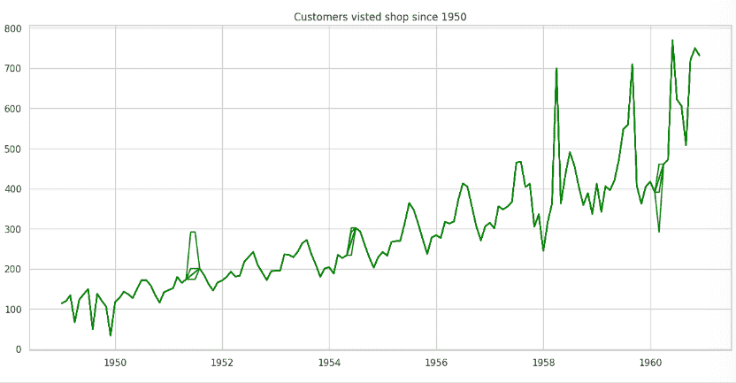
Plot the Graph

This creates a line plot of the data in the DataFrame df. It automatically uses the index (assumed to be the date) as the x-axis and the "Customers" column as the y-axis. 

plt.rcParams['figure.figsize']=(15,7)

plt.plot(df, color='green')

plt.title('Customers visited shop since 1950') 

plt.show()

Output:

Step 4: Imputing the Missing Values

Several techniques can be used to fill missing values in time series data:

1. Mean Imputation: Replaces missing values with the overall average. Simple, but ignores trends.
2. Median Imputation: Uses the median value. More robust to outliers, but still ignores time patterns.
3. Last Observation Carried Forward (LOCF): Fills missing values with the previous known value. Useful for stable trends but may distort changing patterns.
4. Next Observation Carried Backward (NOCB): Uses the next known value. Similar to LOCF but applied backward.
5. Linear Interpolation: Fills gaps by connecting nearby points with a straight line. Works well for smooth trends.
6. Spline Interpolation: Uses a smooth curve to estimate values. Better for complex patterns but more computationally intensive.

1. Mean imputation

• Mean imputation replaces missing values in the "Customers" column with the average of that column.
• A new column named "FillMean" is created, where original values are kept unchanged and missing values are filled with the computed mean.

plt.rcParams['figure.figsize']=(15,7)

df = df.assign(FillMean=df.Customers.fillna(df.Customers.mean()))

plt.plot(df, color='green')

plt.title('Mean Imputation')
plt.show()

Output:

2. Median imputation

• Median imputation replaces missing values in the "Customers" column with the median of that column.
• A new column named "FillMedian" is added, where existing values remain unchanged and missing values are filled using df.Customers.median().

plt.rcParams['figure.figsize']=(15,7)

dataset = df.assign(FillMean=df.Customers.fillna(df.Customers.median()))

plt.plot(dataset, color='green')

plt.title('Median Imputation')
plt.show()

Output:

3. Last Observation Carried Forward(LOCF)

• LOCF fills missing values in the "Customers" column by carrying forward the last available observation.
• In this method, each missing value is replaced with the previous known value and the updated time series can then be visualized to observe the effect.

plt.rcParams['figure.figsize']=(15,7)

df['Customers_locf']= df['Customers'].fillna(method ='ffill')

plt.plot(df['Customers_locf'], color='green')

plt.title('Last Observation Carried Forward')
plt.show()

Output:

4. Next Observation Carried Backward(NOCB)

• NOCB fills missing values in the "Customers" column by using the next available observation.
• Each missing value is replaced with the following known value and the updated time series can be visualized to analyze the impact of this method.

plt.rcParams['figure.figsize']=(15,7)

df['Customers_nocb']= df['Customers'].fillna(method ='bfill')

plt.plot(df['Customers_nocb'], color='green')

plt.title('Next Observation Carried Backward')
plt.show()

Output:

5. Linear Interpolation

• Linear interpolation fills missing values in the "Customers" column by estimating them based on nearby known data points.
• It connects surrounding values with a straight line and uses that line to compute the missing entries.

plt.rcParams['figure.figsize']=(15,7)

df['Customers_L']= df['Customers'].interpolate(method='linear')

plt.plot(df['Customers_L'], color='green')

plt.title('Linear interpolation')
plt.show()

Output:

6. Spline Interpolation

• Spline interpolation fills missing values in the "Customers" column by fitting a smooth curve through the existing data points.
• This method captures more complex patterns than linear interpolation and provides smoother estimates for missing values.

plt.rcParams['figure.figsize']=(15,7)

df['Customers_Spline'] = df['Customers'].interpolate(method='spline', order=3)

plt.plot(df['Customers_Spline'], color='green')

plt.title('Spline Interpolation')
plt.show()

Output: