Window functions in PySpark allow you to perform calculations across a group of rows, returning results for each row individually. They are widely used for data transformations, ranking and analytics.
Types of Window Functions:
- Analytical Function: e.g., lead(), lag(), cume_dist()
- Ranking Function: e.g., row_number(), rank(), dense_rank(), percent_rank()
- Aggregate Function: e.g., avg(), sum(), min(), max()
Analytical Functions
Analytical functions are window functions that return a value for each row based on a group of rows defined by a window. Below is the Sample DataFrame for Analytical Functions.
from pyspark.sql.window import Window
import pyspark
from pyspark.sql import SparkSession

spark = SparkSession.builder.appName("pyspark_window").getOrCreate()
sampleData = (("Olivia", 28, "Sales", 3000),
              ("Harry", 33, "Sales", 4600),
              ("Smith", 40, "Sales", 4100),
              ("Marry", 25, "Finance", 3000),
              ("Henry", 28, "Sales", 3000),
              ("Lars", 46, "Management", 3300),
              ("Jeny", 26, "Finance", 3900),
              ("Aya", 30, "Marketing", 3000),
              ("Omar", 29, "Marketing", 2000),
              ("Johnny", 39, "Sales", 4100)
              )

columns = ["Employee_Name", "Age", "Department", "Salary"]

df = spark.createDataFrame(data=sampleData, schema=columns)

windowPartition = Window.partitionBy("Department").orderBy("Age")
df.printSchema()

df.show()
Output
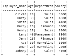
1. Cumulative Distribution
cume_dist() window function is used to get the cumulative distribution within a window partition. It is similar to CUME_DIST in SQL.
from pyspark.sql.functions import cume_dist
df.withColumn("cume_dist",cume_dist().over(windowPartition)).show()
Output
In the output, we can see that a new column is added to the df named "cume_dist" that shows the cumulative distribution value of each row within its Department partition based on the ordering by Age.
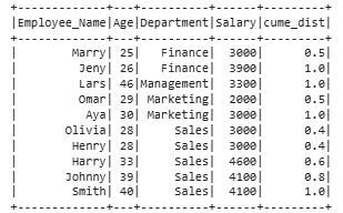
2. Lag Function
lag() function is used to access previous rows' data as per the defined offset value in the function. This function is similar to the LAG in SQL.
from pyspark.sql.functions import lag
df.withColumn("Lag", lag("Salary", 2).over(windowPartition)).show()
Output
In this output, the lag column shows the Salary from 2 rows above, with the first 2 rows as null due to the offset.
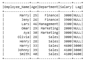
3. Lead Function
lead() function is used to access next rows data as per the defined offset value in the function. This function is similar to the LEAD in SQL and just opposite to lag() function or LAG in SQL.
from pyspark.sql.functions import lead
df.withColumn("Lead", lead("Salary", 2).over(windowPartition)) \
  .show()
Output
Ranking Functions
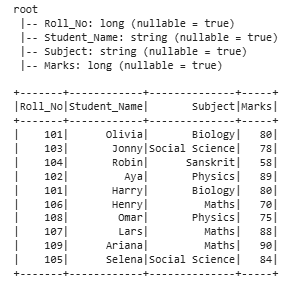
This function assigns a rank or row number to each row within a group or partition, based on the order defined in the window. Examples include row_number(), rank(), and dense_rank(). Below is the Sample Dataframe for demonstration:
from pyspark.sql.window import Window
import pyspark

from pyspark.sql import SparkSession
spark = SparkSession.builder.appName("pyspark_window").getOrCreate()

sampleData = ((101, "Olivia", "Biology", 80),
              (103, "Jonny", "Social Science", 78),
              (104, "Robin", "Sanskrit", 58),
              (102, "Aya", "Physics", 89),
              (101, "Harry", "Biology", 80),
              (106, "Henry", "Maths", 70),
              (108, "Omar", "Physics", 75),
              (107, "Lars", "Maths", 88),
              (109, "Ariana", "Maths", 90),
              (105, "Selena", "Social Science", 84)
              )

columns = ["Roll_No", "Student_Name", "Subject", "Marks"]
df2 = spark.createDataFrame(data=sampleData,
                            schema=columns)

windowPartition = Window.partitionBy("Subject").orderBy("Marks")
df2.printSchema()
df2.show()
Output
1. Row Number
row_number() assigns a sequential number to each row within each window partition based on the specified ordering.
from pyspark.sql.functions import row_number
df2.withColumn("row_number",
               row_number().over(windowPartition)).show()
Output
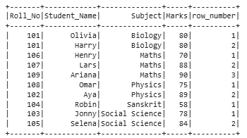
In this output, we can see that we have the row number for each row based on the specified partition i.e. the row numbers are given followed by the Subject and Marks column.
2. Rank
The rank function is used to give ranks to rows specified in the window partition. This function leaves gaps in rank if there are ties.
from pyspark.sql.functions import rank
df2.withColumn("rank", rank().over(windowPartition)) \
    .show()
Output
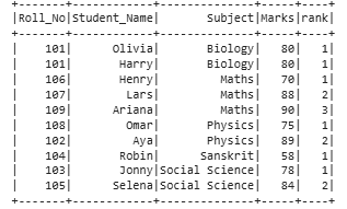
In the output, the rank is provided to each row as per the Subject and Marks column as specified in the window partition.
3. Percent Rank
percent_rank() returns a normalized rank between 0 and 1 based on row position within the partition.. Let's see the example:
from pyspark.sql.functions import percent_rank

df2.withColumn("percent_rank",
               percent_rank().over(windowPartition)).show()
Output
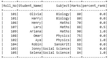
We can see that in the output the rank column contains values in a percentile form i.e. in the decimal format.
4. Dense rank
dense_rank() assigns ranks without gaps when there are ties, unlike rank() which skips rank numbers after ties.
from pyspark.sql.functions import dense_rank
df2.withColumn("dense_rank",
               dense_rank().over(windowPartition)).show()
Output
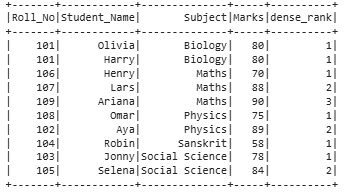
In the output, we can see that the ranks are given in the form of row numbers.
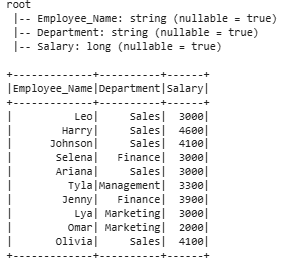
Aggregate function
An aggregate function performs calculations on a group of rows to produce a single summary value, such as AVERAGE, SUM, MIN, or MAX. Below is the Sample Dataframe for demonstration:
import pyspark
from pyspark.sql import SparkSession

spark = SparkSession.builder.appName("pyspark_window").getOrCreate()

sampleData = (("Leo", "Sales", 3000),
              ("Harry", "Sales", 4600),
              ("Johnson", "Sales", 4100),
              ("Selena", "Finance", 3000),
              ("Ariana", "Sales", 3000),
              ("Tyla", "Management", 3300),
              ("Jenny", "Finance", 3900),
              ("Lya", "Marketing", 3000),
              ("Omar", "Marketing", 2000),
              ("Olivia", "Sales", 4100)
              )

columns = ["Employee_Name", "Department", "Salary"]
df3 = spark.createDataFrame(data=sampleData, schema=columns)
df3.printSchema()
df3.show()
Output
Below code computes window aggregates (avg, sum, min, max) of Salary per Department using a partitioned window and adds the results as new columns:
from pyspark.sql.window import Window
from pyspark.sql.functions import col,avg,sum,min,max,row_number

windowPartitionAgg  = Window.partitionBy("Department")
df3.withColumn("Avg", avg(col("Salary")).over(windowPartitionAgg))
  .withColumn("Sum", sum(col("Salary")).over(windowPartitionAgg))
  .withColumn("Min", min(col("Salary")).over(windowPartitionAgg))
  .withColumn("Max", max(col("Salary")).over(windowPartitionAgg)).show()
Output
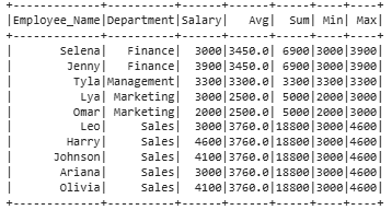
In the output, four new columns Average, Sum, Minimum, and Maximum of Salary are added to 'df3', showing the aggregate values for each row.
