Clinical Trials and outcome analysis are necessary to understand the new effective treatment methods and how they can be used for the public and medical advances. This usually involves the statistical analysis and interpretations of the outcomes. R is a powerful statistical programming language popularly known for such analysis because of its wide range of libraries and packages. This article will explore the study of clinical trial outcomes using R Programming Language.
COVID-19 Clinical Trials Analysis
The dataset consists of 5783 observations and 27 variables related to clinical trials like the status of the trial, available study results, medical conditions, gender, age, sex, type of study, etc. Using this dataset we will analyze the clinical trial outcomes and how they help us in medical and research.
Dataset Link: COVID-19 Clinical Trials Analysis
Load the dataset and libraries
We will use two libraries dplyr and ggplot for data analysis and visualization of graphs. Make sure to change the path of the data with the original one on your PC.
# Load necessary libraries
library(dplyr)
library(ggplot2)

# Load the dataset
data <- read.csv("path_to_dataset.csv")

# Display the first few rows of the dataset
head(data)
Output:
Rank  NCT.Number
1    1 NCT04785898
2    2 NCT04595136
3    3 NCT04395482
4    4 NCT04416061
5    5 NCT04395924
6    6 NCT04516954
                                                                            Title
1                  Diagnostic Performance of the ID Now™ COVID-19 Screening Test Versus Simplexa™ COV
3                                                                Lung CT Scan Analysis of SARS-CoV2 Induced Lung Injury
4                                                    The Role of a Private Hospital in Hong Kong Amid COVID-19 Pandemic
5                                                                            Maternal-foetal Transmission of SARS-Cov-2
6                                                                             Convalescent Plasma for COVID-19 Patients
       Acronym                  Status        Study.Results
1  COVID-IDNow  Active, not recruiting No Results Available
2     COVID-19      Not yet recruiting No Results Available
3  TAC-COVID19              Recruiting No Results Available
4     COVID-19  Active, not recruiting No Results Available
5 TMF-COVID-19              Recruiting No Results Available
6         CPCP Enrolling by invitation No Results Available
                                                 Conditions
1                                                   Covid19
2                                      SARS-CoV-2 Infection
3                                                   covid19
4                                                     COVID
5 Maternal Fetal Infection Transmission|COVID-19|SARS-CoV 2
6                                                  COVID 19

5 Diagnostic Test: Diagnosis of SARS-Cov2 by RT-PCR an
6

1  ....
 Gender                                         Age          Phases Enrollment
1    All   18 Years and older   (Adult, Older Adult)  Not Applicable       1000
2    All   18 Years and older   (Adult, Older Adult) Phase 1|Phase 2         60
3    All   18 Years and older   (Adult, Older Adult)                        500
4    All                   Child, Adult, Older Adult                       2500
5 Female              18 Years to 48 Years   (Adult)                         50
6    All 18 Years to 75 Years   (Adult, Older Adult)   Early Phase 1         10
  Funded.Bys     Study.Type
1      Other Interventional
2      Other Interventional
3      Other  Observational
4   Industry  Observational
5      Other  Observational
6      Other Interventional ....
Data Preprocessing
In this step, we look for the missing values in our dataset so that they do not alter our outcomes.
# Check for missing values
colSums(is.na(data))

# Remove rows with missing values
data <- na.omit(data)
Output:
                   Rank              NCT.Number                   Title
                      0                       0                       0
                Acronym                  Status           Study.Results
                      0                       0                       0
             Conditions           Interventions        Outcome.Measures
                      0                       0                       0
  Sponsor.Collaborators                  Gender                     Age
                      0                       0                       0
                 Phases              Enrollment              Funded.Bys
                      0                      34                       0
             Study.Type           Study.Designs               Other.IDs
                      0                       0                       0
             Start.Date Primary.Completion.Date         Completion.Date
                      0                       0                       0
           First.Posted    Results.First.Posted      Last.Update.Posted
                      0                       0                       0
              Locations         Study.Documents                     URL
                      0                       0                       0
Visualization of the Clinical Trial Outcome data
We will plot the age distribution of the all the participants.
# Age distribution
ggplot(data, aes(x = as.numeric(gsub(" Years and older.*", "", Age)))) +
  geom_histogram(binwidth = 5, fill = "green", color = "black") +
  labs(title = "Age Distribution of Participants", x = "Age", y = "Frequency")
Output:

Comparing Treatment Outcomes
Use statistical tests to compare the outcomes of different treatment groups.
# Convert relevant columns to factors
data$Phases <- as.factor(data$Phases)
data$Status <- as.factor(data$Status)
data$Study.Type <- as.factor(data$Study.Type)
# Summary statistics for Enrollment by Study Type
enrollment_summary <- data %>%
group_by(Study.Type) %>%
summarize(mean_enrollment = mean(Enrollment, na.rm = TRUE))
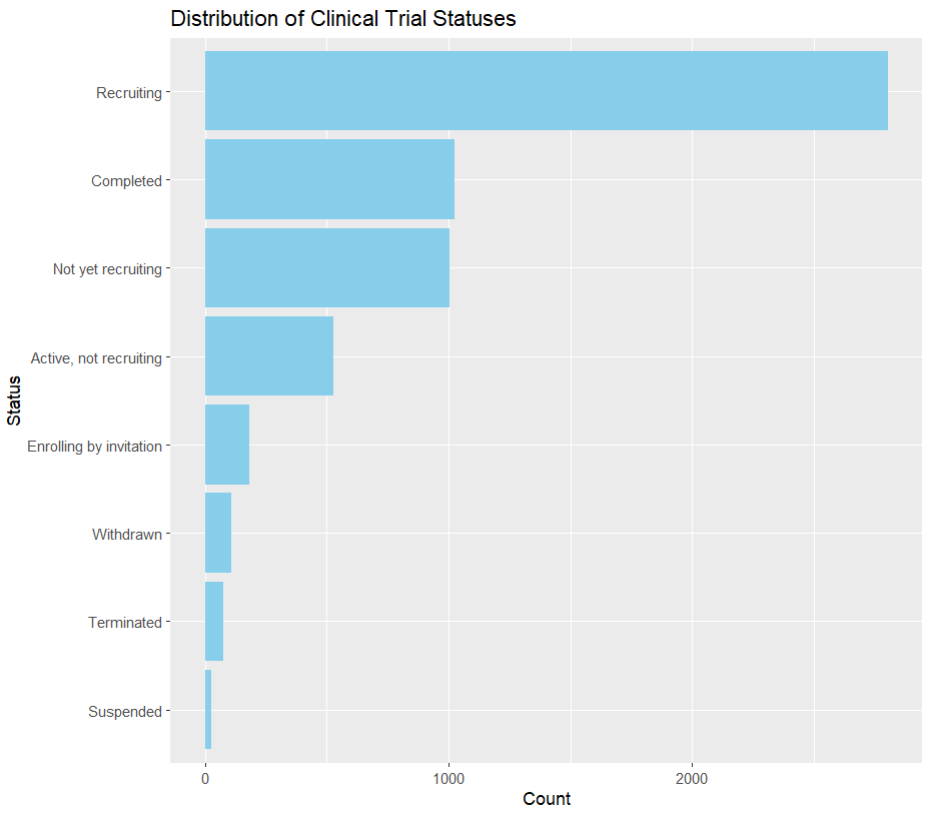
# Count of each status
status_counts <- data %>%
count(Status)
# Bar plot of trial statuses
ggplot(status_counts, aes(x = reorder(Status, n), y = n)) +
geom_bar(stat = "identity", fill = "skyblue") +
coord_flip() +
labs(title = "Distribution of Clinical Trial Statuses", x = "Status", y = "Count")
Output:
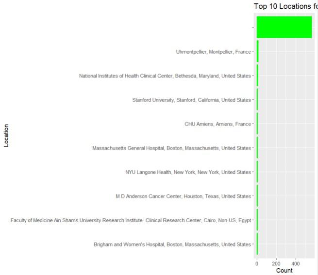
Geographical Distribution of the Trials
Examining the geographical distribution can highlight the global reach and regional focus of clinical trials which is important in a disease like COVID-19 because it is spreads easily with contact.
# Count of trials by location
location_counts <- data %>%
  count(Locations) %>%
  arrange(desc(n)) %>%
  head(10) # Top 10 locations

# Bar plot of top trial locations
ggplot(location_counts, aes(x = reorder(Locations, n), y = n)) +
  geom_bar(stat = "identity", fill = "green") +
  coord_flip() +
  labs(title = "Top 10 Locations for Clinical Trials", x = "Location", y = "Count")
Output:
Analysis of Gender Distribution Across the Trials
Understanding the gender distribution in clinical trials is important for assessing the inclusivity and diversity of the research.
# Count of trials by gender
gender_counts <- data %>%
  count(Gender)

# Bar plot of gender distribution
ggplot(gender_counts, aes(x = reorder(Gender, n), y = n)) +
  geom_bar(stat = "identity", fill = "red") +
  coord_flip() +
  labs(title = "Gender Distribution in Clinical Trials", x = "Gender", y = "Count")
Output:
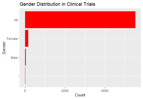
Here, we can see women were more than men in the clinical trials so they dominate in the results obtained. This should be taken care as the anatomy is different men, women and other gender.
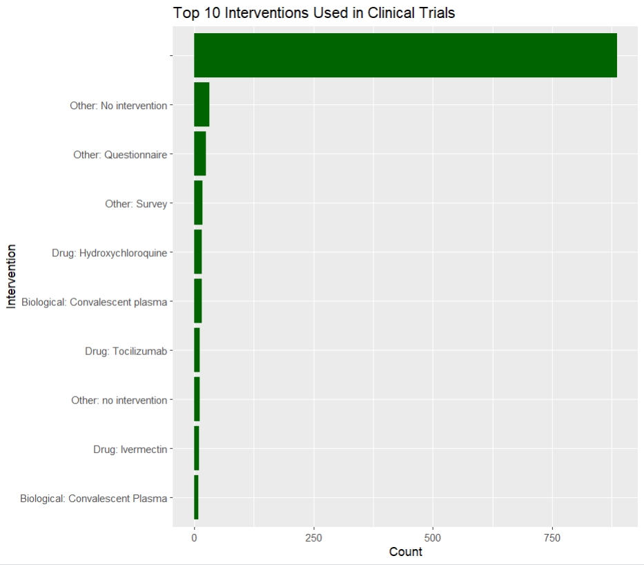
Analysis of Interventions Used in the Clinical Trials
Identifying the most common interventions can reveal the types of treatments being tested.
# Count of trials by intervention
intervention_counts <- data %>%
  count(Interventions) %>%
  arrange(desc(n)) %>%
  head(10) # Top 10 interventions

# Bar plot of top interventions
ggplot(intervention_counts, aes(x = reorder(Interventions, n), y = n)) +
  geom_bar(stat = "identity", fill = "darkgreen") +
  coord_flip() +
  labs(title = "Top 10 Interventions Used in Clinical Trials", x = "Intervention",
                                                               y = "Count")
Output:
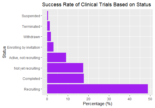
Success Rate of Clinical Trials Based on Their Status
Understanding the success rate (completion rate) of clinical trials based on their status can provide insights into the efficiency and outcomes of clinical research.
# Calculate the success rate
status_counts <- data %>%
  count(Status) %>%
  mutate(percentage = n / sum(n) * 100)

# Bar plot of trial statuses with success rates
ggplot(status_counts, aes(x = reorder(Status, -percentage), y = percentage)) +
  geom_bar(stat = "identity", fill = "purple") +
  coord_flip() +
  labs(title = "Success Rate of Clinical Trials Based on Status", x = "Status",
                                                                  y = "Percentage (%)")
Output:
Patient Outcome Analysis
Patient outcomes are critical indicators of the effectiveness and safety of clinical interventions. Analyzing patient outcomes in clinical trials can provide insights into the efficacy of treatments, side effects, and overall patient health improvements. There are many parameters that we can use to improve the effectiveness and efficiency of the clinical trials:
- Focus on Successful Interventions: Trials with high success rates should be prioritized and taken into further research and development.
- Enhance Outcome Reporting: To improve the quality of the trials they must be reported consistently and continuously. The outcome measures should be well defined.
- Patient-Centric Outcomes: Parameters that directly pay attention to the treatment of the patient should be taken into account such as symptom relief, functional improvements, and survival rates.
Conclusion
This article discussed the clinical trial outcome analysis and how it helps in medicine and research domain. We discussed how packages in R language help us in analysis and visualization of our results for better understanding.
