Pokémon is more than a popular franchise. It is also a rich dataset full of patterns and insights. The data includes attributes such as HP, attack, defense, special stats, types, generation, and whether a Pokémon is legendary.
Dataset Overview
The dataset encompasses detailed attributes for each Pokémon, including:
- Name: The Pokémon's name.
- Type 1 & Type 2: Primary and secondary elemental types.
- Total: Sum of all base stats.
- HP: Hit Points, indicating health.
- Attack & Defense: Physical attack and defense stats.
- Special Attack & Special Defense: Stats for special moves.
- Speed: Determines move order in battles.
- Generation: The generation in which the Pokémon was introduced.
- Legendary Status: Indicates if a Pokémon is legendary
Dataset Link: Pokemon dataset
Installing the Necessary Libraries
We will install and load the packages that we will use like ggplot2 , gridExtra and plotly using the install.packages() function and library() function.
install.packages("ggplot2")
install.packages("gridExtra")
install.packages("plotly")

library(ggplot2)
library(gridExtra)
library(plotly)
Exploring the Dataset
We will now load our dataset and explore it contents , using various functions and statistical methods.
1. Loading the Data
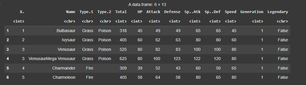
We will read our dataset , which is the Pokemon.csv file using the function read.csv() function and display it first few rows.
pokemon_data <- read.csv("Pokemon.csv")

head(pokemon_data)
Output:
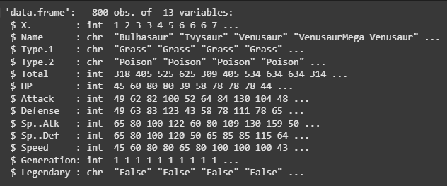
2. Using str() function
To display the pokemon_data data frame structure, the str function is used. The names and data types of each column, such as numerics, numbers, characters or factors, shall also be printed. This also gives insight into data organisation as a whole.
str(pokemon_data)
Output:
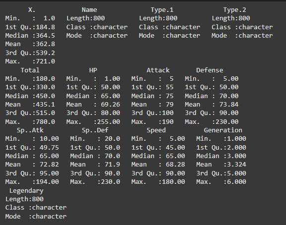
3. Using summary() function
Summarizing the dataset: The summary function shows a summary of the data, such as: statistics of numeric columns, mean, median, quartile, minimum, maximum and frequency counts.
summary(pokemon_data)
Output:
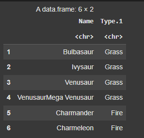
4. Explore specific columns
These lines of code gives the output of the names of the particular pokemon and their primary types.
head(pokemon_data[c('Name','Type.1')])
Output:
Various Visualizations of pokemon data
We will now plot various visualizations to explore the dataset further.
1. Histogram
This line of code shown the histogram of the attack column of the pokemon data.
hist(pokemon_data$Attack)
Output:

2. Bar Plot
This line of code shows the of bar plot , giving count for different types of pokemon (type.1).
type_distribution <- table(pokemon_data$Type.1)

barplot(type_distribution, main = "Distribution of Pokemon Types",
        xlab = "Type", ylab = "Count", col = rainbow(length(type_distribution)))
Output:

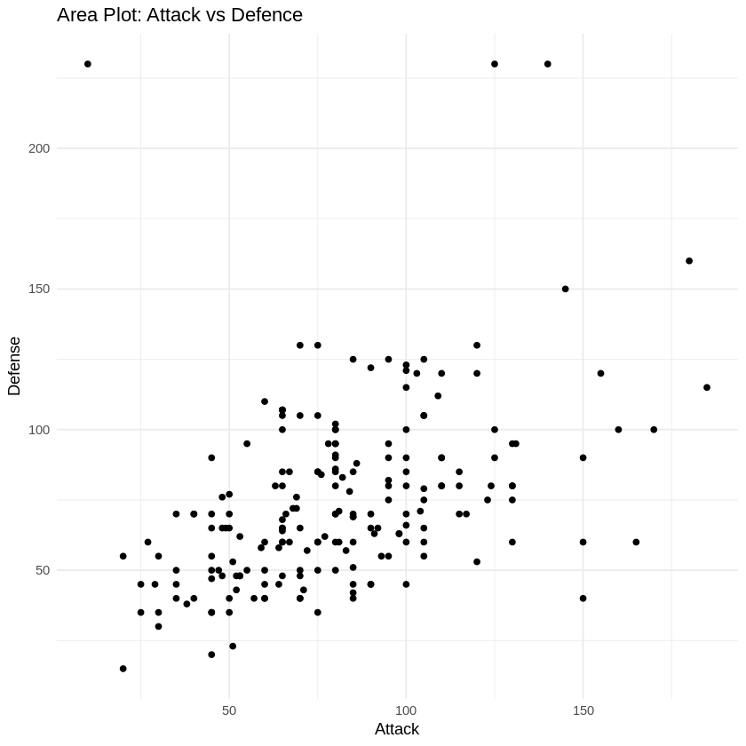
3. Scatter Plot
This code generates individual scatter plots for each pair of attributes (Attack vs Defence) with color-coding based on Pokémon types. This approach should be more manageable in terms of computation time. Adjustments can be made based on your specific needs and preferences.
selected_pokemon <- pokemon_data[sample(1:nrow(pokemon_data), 200), ]

scatter_plots <- ggplot(selected_pokemon, aes(x = Attack, y = Defense)) +
    geom_point() +
    labs(title = "Area Plot: Attack vs Defence") +
    theme_minimal()

scatter_plots
Output:
4. Pie Chart
A quick glance at the ratio of legendary to unlegendary Pokémon can be found using a pie chart.
legendary_distribution <- table(pokemon_data$Legendary)
pie(legendary_distribution, main = "Proportion of Legendary Pokemon",
    labels = c("Non-Legendary", "Legendary"), col = c("skyblue", "lightcoral"))
Output:
.png)
5. Box Plot
We will create box plots for each pair of attributes (Sp..Def and Sp..Atk) for some selected pokemons.
selected_pokemon <- pokemon_data[sample(1:nrow(pokemon_data), 800), ]

box_plots <- list(
  ggplot(selected_pokemon, aes(x = Sp..Atk, y = Sp..Def, color = Type.1)) +
    geom_boxplot()+
    labs(title = "Box plot: Sp.Attack and Sp.Defense")+
    theme_minimal()

)

grid.arrange(grobs = box_plots, ncol = 1)
Output:

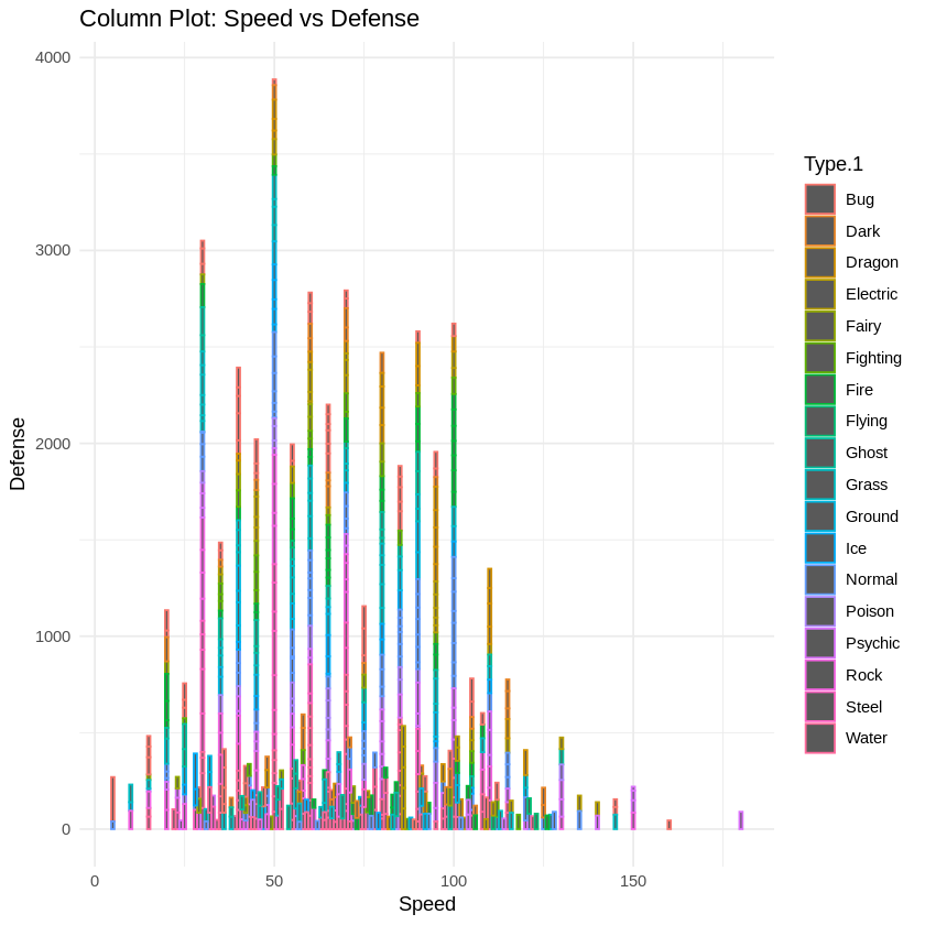
6. Column Plot
We will create a column plot to showcase speed vs defence for the different type1 pokemons.
scatter_plots <- list(
  ggplot(pokemon_data, aes(x = Speed, y = Defense, color = Type.1)) +
    geom_col()+
    labs(title = "Column Plot: Speed vs Defense") +
    theme_minimal()

)
grid.arrange(grobs = scatter_plots, ncol = 1)
Output:
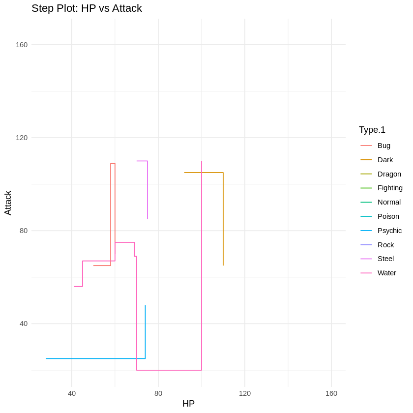
7. Step Plot
We randomly select 50 Pokémon from the dataset to simplify visualization. A step plot is then created using ggplot2 to show how Attack varies with HP, colored by the primary type (Type.1). The plot is displayed using grid.arrange(), allowing easy expansion for more plots later.
selected_pokemon <- pokemon_data[sample(1:nrow(pokemon_data), 50), ]

scatter_plots <- list(
  ggplot(selected_pokemon, aes(x = HP, y = Attack, color = Type.1)) +
    geom_step()+
    labs(title = "Step Plot: HP vs Attack") +
    theme_minimal()

)
grid.arrange(grobs = scatter_plots, ncol = 1)
Output:
In this article, we explored the rich dataset of Pokémon attributes using R, uncovering patterns and insights through various visualizations and analyses. From examining basic distributions to creating advanced plots, we demonstrated how this data can be used to understand relationships between features. This sets the stage for further exploration, such as clustering similar Pokémon or building predictive models for battle outcomes.
