Visualizing the Kolmogorov-Smirnov Statistic in ggplot2 Using R

In this article, we will explore how to visualize the K-S statistic in R using the ggplot2 package. We will demonstrate how to perform the K-S test and then visualize the empirical and theoretical cumulative distribution functions along with the K-S statistic using R Programming Language.

What is Kolmogorov-Smirnov?

The Kolmogorov-Smirnov (K-S) test is a non-parametric test used to compare two distributions or a sample against a reference distribution. The K-S statistic quantifies the distance between the empirical distribution function of the sample and the cumulative distribution function of the reference distribution. Visualizing the K-S statistic can help in understanding the differences between these distributions.

To follow along, you need to have the following R packages installed:

• ggplot2: For creating the plots.
• stats: For performing the Kolmogorov-Smirnov test.

Let's create a sample dataset and perform the K-S test to compare it against a theoretical normal distribution.

# Load necessary library
library(ggplot2)

# Set seed for reproducibility
set.seed(123)

# Generate a sample of 100 observations from a normal distribution
sample_data <- rnorm(100, mean = 0, sd = 1)

# Perform the Kolmogorov-Smirnov test
ks_test <- ks.test(sample_data, "pnorm", mean = 0, sd = 1)
ks_test

Output:

	Asymptotic one-sample Kolmogorov-Smirnov test

data:  sample_data
D = 0.093034, p-value = 0.3522
alternative hypothesis: two-sided

• rnorm(100, mean = 0, sd = 1): Generates 100 random observations from a normal distribution with mean 0 and standard deviation 1.
• ks.test(sample_data, "pnorm", mean = 0, sd = 1): Performs the K-S test to compare the sample against the standard normal distribution.

The output of the K-S test will provide the K-S statistic and the p-value, which indicates whether the sample distribution differs significantly from the theoretical distribution.

Visualizing the Empirical and Theoretical CDFs

To visualize the K-S statistic, we need to plot the empirical cumulative distribution function (ECDF) of the sample data and the cumulative distribution function (CDF) of the reference normal distribution.

# Create a data frame for plotting
plot_data <- data.frame(
  x = sort(sample_data),
  ecdf = ecdf(sample_data)(sort(sample_data)),
  cdf = pnorm(sort(sample_data), mean = 0, sd = 1)
)

# Calculate the K-S statistic line
ks_line <- data.frame(
  x = c(ks_test$statistic, ks_test$statistic),
  y = c(pnorm(ks_test$statistic, mean = 0, sd = 1), ecdf(sample_data)(ks_test$statistic))
)

# Plot the ECDF and theoretical CDF
ggplot(plot_data, aes(x = x)) +
  geom_line(aes(y = ecdf), color = "blue", size = 1, linetype = "solid") +
  geom_line(aes(y = cdf), color = "red", size = 1, linetype = "dashed") +
  geom_segment(data = ks_line, aes(x = x[1], xend = x[2], y = y[1], yend = y[2]),
               color = "purple", linetype = "dotted", size = 1.5) +
  labs(title = "Kolmogorov-Smirnov Test: ECDF vs Theoretical CDF",
       x = "Value",
       y = "Cumulative Probability") +
  theme_minimal() +
  theme(plot.title = element_text(hjust = 0.5)) +
  annotate("text", x = ks_test$statistic, y = max(ks_line$y),
           label = paste0("K-S Statistic = ", round(ks_test$statistic, 3)),
           vjust = -1.5, color = "purple")

Output:

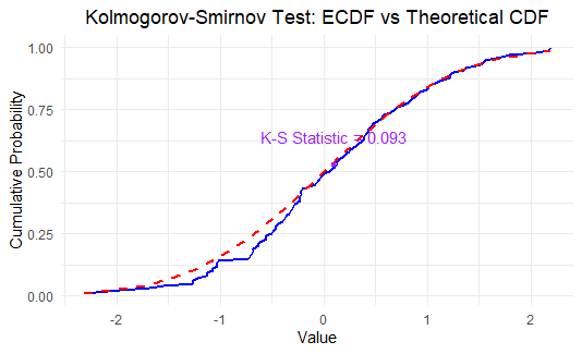
• geom_line(aes(y = ecdf), color = "blue", size = 1, linetype = "solid"): Plots the ECDF of the sample data.
• geom_line(aes(y = cdf), color = "red", size = 1, linetype = "dashed"): Plots the theoretical CDF of the normal distribution.
• geom_segment(data = ks_line, aes(x = x[1], xend = x[2], y = y[1], yend = y[2])): Adds a line segment to represent the K-S statistic (the maximum vertical distance between the ECDF and the theoretical CDF).
• annotate(): Adds a text annotation to display the K-S statistic value on the plot.

Conclusion

Visualizing the Kolmogorov-Smirnov statistic in R using ggplot2 allows you to understand the differences between an empirical distribution and a theoretical distribution. By plotting the ECDF and the CDF together and highlighting the K-S statistic, you can clearly see where the maximum deviation occurs. This visualization is a powerful tool for interpreting the results of the K-S test and assessing the fit between your sample data and a reference distribution.