XGBoost (Extreme Gradient Boosting) is a scalable gradient boosting framework that sequentially builds decision trees, where each tree corrects errors of the previous one. It supports parallel processing, L1/L2 regularization and automatic missing value handling, making it faster and more robust than traditional gradient boosting.
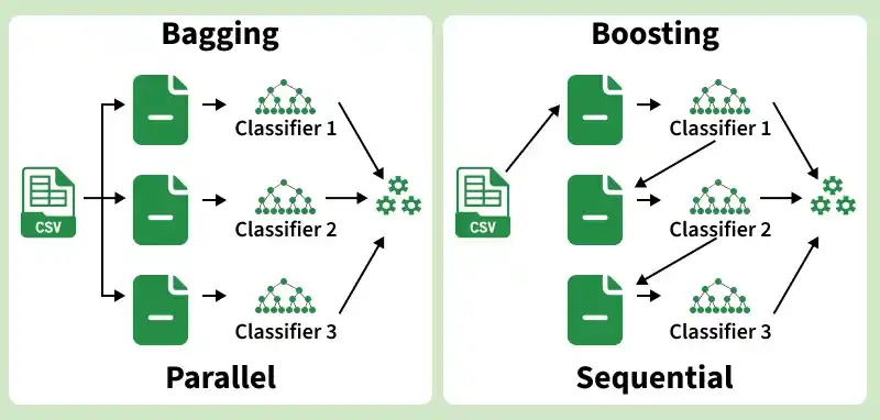
XGBoost modeling is built on two core ensemble techniques:
- Bagging: Randomly samples data to build multiple learning algorithms and combines their outputs to improve stability and accuracy.
- Boosting: Sequentially builds models where each new model focuses more on the observations misclassified by the previous one, progressively improving performance.
How XGBoost Works
XGBoost builds an ensemble of decision trees sequentially, where each new tree focuses on correcting the errors made by the previous one. It optimizes a regularized objective function combining a loss function and a regularization term to prevent overfitting.
- Initialization: The model starts with an initial prediction, typically the mean of the target variable for regression tasks.
- Compute Residuals: The difference between actual and predicted values (residuals) is calculated for each iteration.
- Build a Decision Tree: A new decision tree is fitted on the residuals to capture the remaining errors.
- Update Predictions: The predictions are updated by adding the new tree's output scaled by the learning rate (eta).
- Regularization: L1 and L2 regularization penalties are applied at each step to control model complexity and prevent overfitting.
- Repeat: Steps 2–5 are repeated for a defined number of rounds (nrounds) or until early stopping criteria are met.
- Final Prediction: The output is the sum of predictions from all trees combined.
Parameters of XGBoost
XGBoost provides several key hyperparameters to control model behavior and performance:
param_list = list(
objective = "reg:linear",
eta = 0.01,
gamma = 1,
max_depth = 6,
subsample = 0.8,
colsample_bytree = 0.5
)
- eta: Learning rate (0 to 1) that shrinks feature weights to prevent overfitting. Lower values make the model more conservative, also known as the shrinking factor.
- gamma: Minimum loss reduction required to make a split. Higher values make the algorithm more conservative. Range 0 to infinity.
- max_depth: Maximum depth of each decision tree, controls the complexity of the model.
- subsample: Proportion of training rows randomly sampled to grow each tree.
- colsample_bytree: Ratio of features randomly selected to build each tree.
- objective: Defines the learning task. Here reg:linear is used for regression.
Step By Step Implementation
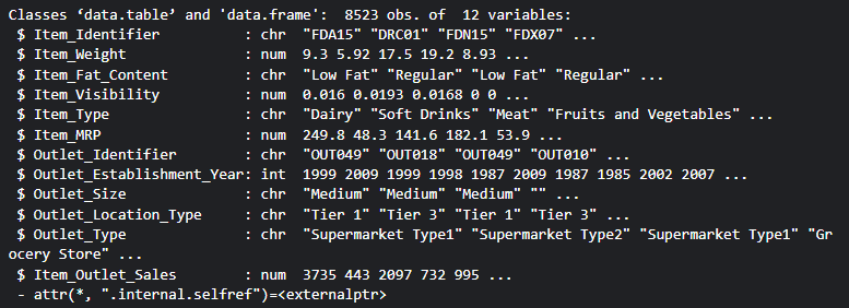
We will demonstrate XGBoost using the Big Mart Sales dataset, which consists of 1,559 products across 10 stores in different cities. The dataset contains 12 features including and Item_Outlet_Sales as the target variable.
Download dataset from here
Step 1: Install and Load Required Packages
Install and load all necessary R libraries for data manipulation, visualization and model building.
install.packages(c("data.table", "dplyr", "ggplot2",
                   "caret", "xgboost", "e1071", "cowplot"))

library(data.table)
library(dplyr)
library(ggplot2)
library(caret)
library(xgboost)
library(e1071)
library(cowplot)
Step 2: Load and Combine Dataset
Load the train and test datasets and combine them for uniform preprocessing.
train = fread("Train_UWu5bXk.csv")
test  = fread("Test_u94Q5KV.csv")
str(train)

test[, Item_Outlet_Sales := NA]
combi = rbind(train, test)
Output:
Step 3: Handle Missing Values
Replace missing values in Item_Weight with the mean weight of the same product and replace zero values in Item_Visibility with the product mean.
# Impute missing Item_Weight
missing_index = which(is.na(combi$Item_Weight))
for(i in missing_index){
  item = combi$Item_Identifier[i]
  combi$Item_Weight[i] = mean(combi$Item_Weight
                        [combi$Item_Identifier == item], na.rm = T)
}

# Replace 0 in Item_Visibility with mean
zero_index = which(combi$Item_Visibility == 0)
for(i in zero_index){
  item = combi$Item_Identifier[i]
  combi$Item_Visibility[i] = mean(combi$Item_Visibility
                        [combi$Item_Identifier == item], na.rm = T)
}
Step 4: Encode Categorical Variables
Since XGBoost works only with numeric variables, convert categorical features using Label Encoding and One Hot Encoding.
# Label Encoding
combi[, Outlet_Size_num := ifelse(Outlet_Size == "Small", 0,
                           ifelse(Outlet_Size == "Medium", 1, 2))]

combi[, Outlet_Location_Type_num := ifelse(Outlet_Location_Type == "Tier 3", 0,
                                    ifelse(Outlet_Location_Type == "Tier 2", 1, 2))]

combi[, c("Outlet_Size", "Outlet_Location_Type") := NULL]

# One Hot Encoding
ohe_1 = dummyVars("~.", data = combi[, -c("Item_Identifier",
                  "Outlet_Establishment_Year", "Item_Type")], fullRank = T)

ohe_df = data.table(predict(ohe_1, combi[, -c("Item_Identifier",
                    "Outlet_Establishment_Year", "Item_Type")]))

combi = cbind(combi[, "Item_Identifier"], ohe_df)
Step 5: Remove Skewness and Scale Data
Apply log transformation to reduce skewness in Item_Visibility, then center and scale all numeric features for better model performance.
# Log transformation to remove skewness
combi[, Item_Visibility := log(Item_Visibility + 1)]

# Scale and center numeric features
num_vars = which(sapply(combi, is.numeric))
num_vars_names = names(num_vars)

combi_numeric = combi[, setdiff(num_vars_names, "Item_Outlet_Sales"), with = F]
prep_num = preProcess(combi_numeric, method = c("center", "scale"))
combi_numeric_norm = predict(prep_num, combi_numeric)

combi[, setdiff(num_vars_names, "Item_Outlet_Sales") := NULL]
combi = cbind(combi, combi_numeric_norm)
Step 6: Split Data Back to Train and Test
After preprocessing, split the combined dataset back into train and test sets.
train = combi[1:nrow(train)]
test  = combi[(nrow(train) + 1):nrow(combi)]
test[, Item_Outlet_Sales := NULL]
Step 7: Define Model Parameters and Convert to XGBoost Format
Define hyperparameters and convert the datasets into xgb.DMatrix format, which is the optimized data structure required by XGBoost.
param_list = list(
  objective        = "reg:linear",
  eta              = 0.01,
  gamma            = 1,
  max_depth        = 6,
  subsample        = 0.8,
  colsample_bytree = 0.5
)

Dtrain = xgb.DMatrix(data = as.matrix(train[, -c("Item_Identifier",
                     "Item_Outlet_Sales")]), label = train$Item_Outlet_Sales)

Dtest  = xgb.DMatrix(data = as.matrix(test[, -c("Item_Identifier")]))
Step 8: Cross-Validation to Find Optimal Rounds
Use 5-fold cross-validation to find the optimal number of boosting rounds before training the final model.
set.seed(112)
xgbcv = xgb.cv(params = param_list,
                data = Dtrain,
                nrounds = 1000,
                nfold = 5,
                print_every_n = 10,
                early_stopping_rounds = 30,
                maximize = F)
Output:
The xgboost model is trained calculating the train-rmse score and test-rmse score and finding its lowest value in many rounds.
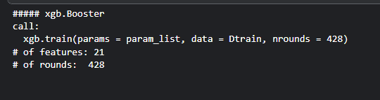
Step 9: Train the Final XGBoost Model
Train the final model using the optimal number of rounds identified from cross-validation.
xgb_model = xgb.train(data = Dtrain,
                      params = param_list,
                      nrounds = 428)
xgb_model
Output:
Step 10: Plot Variable Importance
Identify and visualize the most influential features in the model using the variable importance plot.
var_imp = xgb.importance(feature_names = setdiff(names(train),
                         c("Item_Identifier", "Item_Outlet_Sales")),
                         model = xgb_model)

xgb.plot.importance(var_imp)
Output:
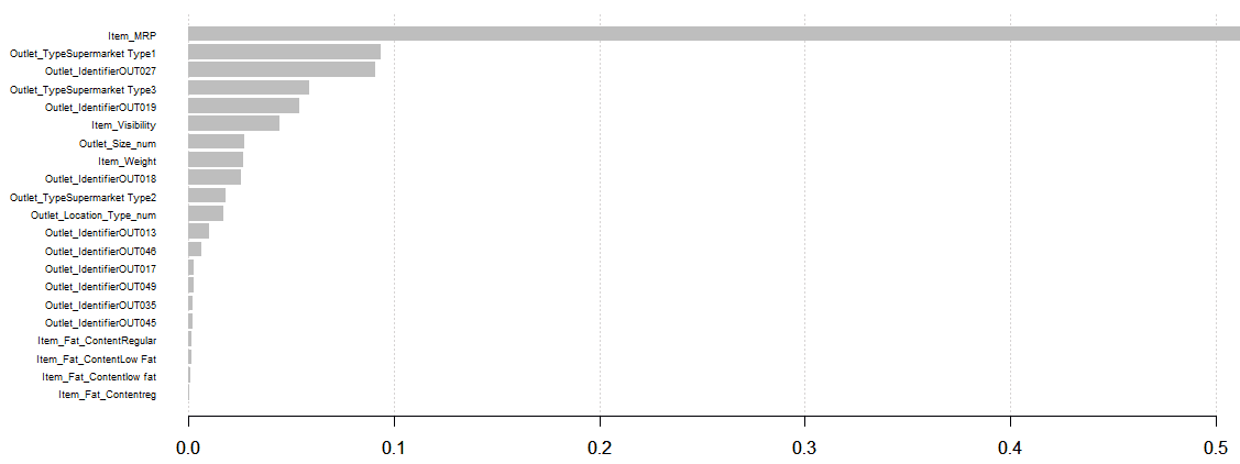
From the variable importance plot, Item_MRP is the most influential feature, suggesting that product pricing and store location are key drivers of sales.
Download full code from here
