The Zipf distribution is an important statistical model that captures the "rank-frequency" relationship in various natural and social phenomena. It describes how a few items are very common, while many items are rare. This article will guide you through understanding, generating, visualizing, and analyzing the Zipf distribution in R Programming Language.
Introduction to Zipf Distribution
The Zipf distribution, named after linguist George Zipf, is a discrete probability distribution often observed in natural language processing, population distributions, website traffic analysis, etc. It states that the frequency of an element is inversely proportional to its rank in a frequency table.
For example, in a typical book, the most frequent word appears twice as often as the second most frequent word, three times as often as the third most frequent word, and so on.
Applications of Zipf Distribution
Zipf distribution appears in many real-world scenarios, such as:
- Natural language processing: Word frequency in texts
- City population sizes: Population rankings of cities
- Website traffic: Visits to websites or pages
- Wealth distribution: Distribution of wealth among people
Step 1: Installing and Loading Required Packages
To work with the Zipf distribution in R, we will use the zipfR package, which offers functionality to work with Zipf distribution models.
# Install the zipfR package
install.packages("zipfR")

# Load the package
library(zipfR)
Step 2: Generating Zipf Distribution Data
Let's generate a Zipf-distributed sample using R. We'll create a sequence of ranks and calculate their probabilities based on a given shape parameter s.
# Load necessary libraries
library(ggplot2)

# Define parameters
N <- 100   # Total number of elements
s <- 1.5   # Shape parameter

# Generate Zipf distribution probabilities
zipf_probs <- (1 / (1:N)^s) / sum(1 / (1:N)^s)
zipf_data <- data.frame(Rank = 1:N, Probability = zipf_probs)

# Display the first few rows
head(zipf_data)
Output:
  Rank Probability
1    1  0.41444351
2    2  0.14652791
3    3  0.07975969
4    4  0.05180544
5    5  0.03706895
6    6  0.02819931
Step 3: Visualizing the Zipf Distribution
We can visualize the Zipf distribution using the ggplot2 package.
# Install and load ggplot2 if not already installed
library(ggplot2)

# Basic Zipf distribution plot
ggplot(zipf_data, aes(x = Rank, y = Probability)) +
  geom_line(color = "blue", size = 1) +
  labs(title = "Basic Zipf Distribution",
       x = "Rank",
       y = "Probability") +
  theme_minimal()
Output:
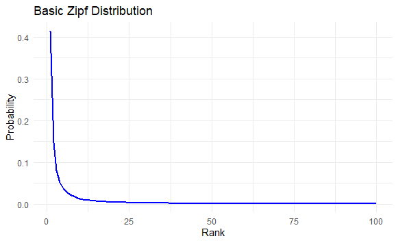
This plot shows a clear decline in probabilities as ranks increase, demonstrating the Zipfian principle.
Step 4: Comparison of Different Shape Parameters
To see how the shape parameter sss affects the Zipf distribution, let's compare multiple values of sss on the same plot.
# Define different shape parameters
shape_params <- c(1.1, 1.5, 2.0)

# Create a data frame for all shape parameters
zipf_data_multi <- data.frame(Rank = integer(), Probability = numeric(), Shape = factor())

for (s in shape_params) {
  zipf_probs <- (1 / (1:N)^s) / sum(1 / (1:N)^s)
  temp_data <- data.frame(Rank = 1:N, Probability = zipf_probs, Shape = as.factor(s))
  zipf_data_multi <- rbind(zipf_data_multi, temp_data)
}

# Plot Zipf distributions for different shape parameters
ggplot(zipf_data_multi, aes(x = Rank, y = Probability, color = Shape)) +
  geom_line(size = 1) +
  labs(title = "Comparison of Zipf Distributions with Different Shape Parameters",
       x = "Rank",
       y = "Probability",
       color = "Shape (s)") +
  theme_minimal() +
  theme(legend.position = "bottom")
Output:
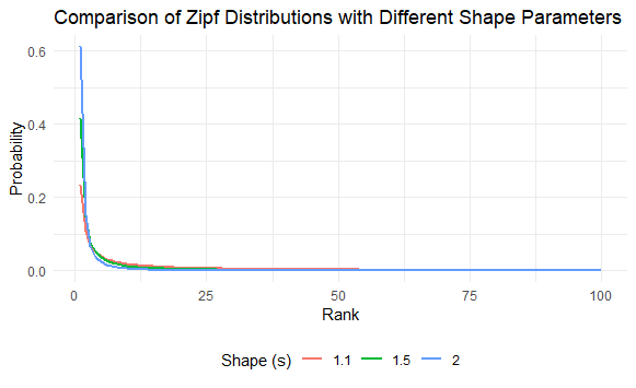
The plot shows how increasing the shape parameter sss leads to a steeper decline in probability.
Fitting a Zipf Distribution to Custom Data
Let's generate data that follows a Zipf distribution and fit a curve to it.
# Generate synthetic data following Zipf distribution
set.seed(123)
N <- 100  # Number of elements
s <- 1.5  # Shape parameter
zipf_sample <- sample(1:N, 1000, replace = TRUE, prob = (1 / (1:N)^s))

# Create a frequency table
zipf_freq_table <- as.data.frame(table(zipf_sample))
colnames(zipf_freq_table) <- c("Rank", "Frequency")
zipf_freq_table$Rank <- as.numeric(as.character(zipf_freq_table$Rank))

# Fit a curve to the observed frequencies
ggplot(zipf_freq_table, aes(x = Rank, y = Frequency)) +
  geom_point(color = "red", size = 2) +
  geom_smooth(method = "lm", formula = y ~ I(1 / x^s), color = "blue", se = FALSE) +
  scale_x_log10() + scale_y_log10() +
  labs(title = "Fitting a Zipf Distribution to Custom Data",
       x = "Rank (Log Scale)",
       y = "Frequency (Log Scale)") +
  theme_minimal()
Output:
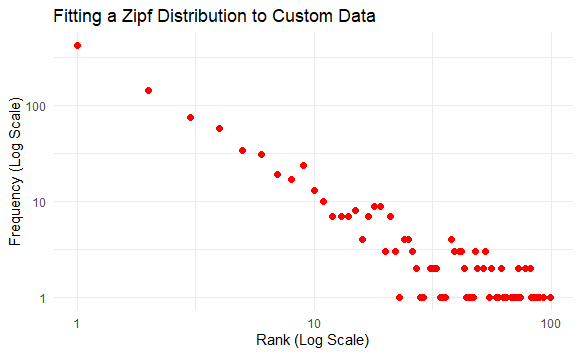
The plot shows how well the Zipf distribution fits the observed data, with a clear alignment on the log-log scale.
Conclusion
The Zipf distribution is a fascinating model that captures the essence of rank-based phenomena across various domains, from linguistics to social sciences. Using R, we can generate, visualize, and analyze the Zipf distribution with ease, making it an excellent tool for data scientists, statisticians, and researchers. Whether you're working on text analysis, city population studies, or any other application where rank-frequency relationships matter, understanding Zipf distribution can provide valuable insights into the underlying data patterns.
