Latent Class Analysis is widely applied in various fields such as psychology, sociology, and epidemiology. In R, several packages provide functions for conducting LCA, with poLCA, flexmix, and Mclust being some of the popular ones.
Latent Class Analysis in R
Latent Class Analysis (LCA) in R Programming Language is a statistical method used to identify unobserved subgroups within a population based on individuals' responses to observed categorical variables. It is widely used in various fields, including psychology, sociology, marketing, and education, to uncover hidden structures and patterns within data. By modeling the probability of membership in latent classes, LCA helps in understanding population heterogeneity and simplifying complex data structures.
Implementing Latent Class Analysis in R
The poLCA package in R provides functions to perform LCA using a finite mixture modeling approach. Below is a step-by-step guide to conduct LCA using poLCA.
Step 1: Installing and Load the required Packages
Now we will install and load the required Packages.
# Install and load the poLCA package
install.packages("poLCA")
library(poLCA)
Step 2: Data Preparation
Prepare your data by ensuring that it is in the appropriate format for LCA. The data should consist of categorical variables representing observed responses.
# Simulated dataset
set.seed(123)
survey_data <- data.frame(
  Q1 = sample(1:3, 1000, replace = TRUE),
  Q2 = sample(1:4, 1000, replace = TRUE),
  Q3 = sample(1:3, 1000, replace = TRUE),
  Q4 = sample(1:4, 1000, replace = TRUE),
  Q5 = sample(1:3, 1000, replace = TRUE)
)
head(survey_data)
Output:
  Q1 Q2 Q3 Q4 Q5
1  3  4  1  4  3
2  3  2  3  1  2
3  3  3  3  1  2
4  2  2  2  4  1
5  3  4  1  2  3
6  2  4  3  2  1
This creates a simulated dataset with 1000 respondents answering 5 questions (Q1 to Q5). The responses are sampled randomly from specified ranges.
Step 3:Model Specification
To specify an LCA model, use the poLCA function from the poLCA package. Define a formula indicating the observed variables and set the number of latent classes we want to extract.
# Specifying the LCA model with 3 latent classes
f <- cbind(Q1, Q2, Q3, Q4, Q5) ~ 1
lca_model <- poLCA(f, survey_data, nclass = 3)
Output:
Conditional item response (column) probabilities,
 by outcome variable, for each class (row)

$Q1
           Pr(1)  Pr(2)  Pr(3)
class 1:  0.2480 0.4188 0.3332
class 2:  0.3746 0.3205 0.3050
class 3:  0.3310 0.2679 0.4011

$Q2
           Pr(1)  Pr(2)  Pr(3)  Pr(4)
class 1:  0.1712 0.0517 0.5381 0.2390
class 2:  0.2215 0.2758 0.2750 0.2278
class 3:  0.3626 0.3964 0.0000 0.2409

$Q3
           Pr(1)  Pr(2)  Pr(3)
class 1:  0.3559 0.2420 0.4020
class 2:  0.2997 0.2923 0.4079
class 3:  0.3595 0.3989 0.2416

$Q4
           Pr(1)  Pr(2)  Pr(3)  Pr(4)
class 1:  0.2073 0.5334 0.0097 0.2497
class 2:  0.2022 0.0474 0.5650 0.1853
class 3:  0.3243 0.3391 0.0019 0.3346

$Q5
           Pr(1)  Pr(2)  Pr(3)
class 1:  0.2819 0.3847 0.3334
class 2:  0.3308 0.3066 0.3625
class 3:  0.3138 0.4112 0.2750

Estimated class population shares
 0.2754 0.4101 0.3144

Predicted class memberships (by modal posterior prob.)
 0.245 0.311 0.444

=========================================================
Fit for 3 latent classes:
=========================================================
number of observations: 1000
number of estimated parameters: 38
residual degrees of freedom: 393
maximum log-likelihood: -6044.248

AIC(3): 12164.5
BIC(3): 12350.99
G^2(3): 462.2892 (Likelihood ratio/deviance statistic)
X^2(3): 397.0556 (Chi-square goodness of fit)

ALERT: iterations finished, MAXIMUM LIKELIHOOD NOT FOUND
The conditional item response probabilities represent the probabilities of observing specific responses (categories) for each item (question) within each latent class.
- $Q1 to $Q5: Each item (question) in the dataset is represented by a separate section. For example, $Q1 corresponds to the first question, $Q2 to the second question, and so on.
- Pr(1) to Pr(4): These columns represent the categories or response options for each question. For example, Pr(1) corresponds to category 1, Pr(2) to category 2, and so on.
- class 1 to class 3: Each row represents a latent class, and the probabilities within each row indicate the likelihood of individuals in that class choosing each response option for the respective question.
The estimated class population shares provide information about the distribution of individuals across the latent classes.
- 0.2754, 0.4101, 0.3144: These values represent the estimated proportions of individuals belonging to each latent class, respectively.
The predicted class memberships indicate the most likely class assignment for each individual based on the modal posterior probability.
- 0.245, 0.311, 0.444: These values represent the proportions of individuals predicted to belong to each latent class, respectively.
The fit statistics assess the adequacy of the model to the observed data.
- AIC (Akaike Information Criterion): A measure of the relative quality of a statistical model, with lower values indicating better fit.
- BIC (Bayesian Information Criterion): Similar to AIC but penalizes model complexity more heavily, with lower values indicating better fit.
- G^2 (Likelihood Ratio/Deviance Statistic): A goodness-of-fit statistic based on the difference between the observed and expected frequencies, with smaller values indicating better fit.
- X^2 (Chi-square Goodness of Fit): Another goodness-of-fit statistic based on the chi-square distribution, with smaller values indicating better fit.
- Maximum Log-Likelihood: Represents the maximum value of the log-likelihood function achieved during model estimation.
- Iterations Finished, Maximum Likelihood Not Found: Indicates that the iterative estimation process converged, but the maximum likelihood value was not found. This may suggest potential issues with model convergence.
Overall, the fit statistics suggest that the model with 3 latent classes adequately describes the observed data, as indicated by relatively low AIC and BIC values and reasonable goodness-of-fit statistics. However, the alert regarding the maximum likelihood not being found warrants further investigation into the convergence of the estimation process.
Step 4: Estimation Methods
The poLCA function uses the Expectation-Maximization (EM) algorithm to estimate model parameters. This iterative method maximizes the likelihood of the data given the model. By default, poLCA initializes the EM algorithm with multiple random starts to avoid local maxima.
# Fitting the model with multiple random starts
lca_model <- poLCA(f, survey_data, nclass = 3, nrep = 5)
Output:
Model 1: llik = -6044.317 ... best llik = -6044.317
Model 2: llik = -6044.172 ... best llik = -6044.172
Model 3: llik = -6044.023 ... best llik = -6044.023
Model 4: llik = -6044.239 ... best llik = -6044.023
Model 5: llik = -6044.085 ... best llik = -6044.023
Conditional item response (column) probabilities,
 by outcome variable, for each class (row)

$Q1
           Pr(1)  Pr(2)  Pr(3)
class 1:  0.3065 0.2906 0.4029
class 2:  0.3746 0.3145 0.3109
class 3:  0.1756 0.4752 0.3492

$Q2
           Pr(1)  Pr(2)  Pr(3)  Pr(4)
class 1:  0.3899 0.3527 0.0000 0.2574
class 2:  0.2220 0.2655 0.2852 0.2273
class 3:  0.0956 0.0000 0.6838 0.2206

$Q3
           Pr(1)  Pr(2)  Pr(3)
class 1:  0.3722 0.3875 0.2403
class 2:  0.2979 0.2966 0.4055
class 3:  0.3987 0.2225 0.3789

$Q4
           Pr(1)  Pr(2)  Pr(3)  Pr(4)
class 1:  0.3081 0.3336 0.0001 0.3582
class 2:  0.2337 0.1577 0.4150 0.1937
class 3:  0.1436 0.6016 0.0001 0.2547

$Q5
           Pr(1)  Pr(2)  Pr(3)
class 1:  0.3110 0.4326 0.2564
class 2:  0.3331 0.3126 0.3543
class 3:  0.2318 0.4076 0.3606

Estimated class population shares
 0.2883 0.5662 0.1456

Predicted class memberships (by modal posterior prob.)
 0.363 0.518 0.119

=========================================================
Fit for 3 latent classes:
=========================================================
number of observations: 1000
number of estimated parameters: 38
residual degrees of freedom: 393
maximum log-likelihood: -6044.023

AIC(3): 12164.05
BIC(3): 12350.54
G^2(3): 461.8389 (Likelihood ratio/deviance statistic)
X^2(3): 397.9841 (Chi-square goodness of fit)

ALERT: iterations finished, MAXIMUM LIKELIHOOD NOT FOUND
It suggest that the model with 3 latent classes adequately describes the observed data, as indicated by relatively low AIC and BIC values and reasonable goodness-of-fit statistics. However, the alert regarding the maximum likelihood not being found warrants further investigation into the convergence of the estimation process.
Step 5: Model Selection
Choosing the optimal number of latent classes is crucial. Fit multiple models with different numbers of classes and compare their fit using criteria such as the Bayesian Information Criterion (BIC) and Akaike Information Criterion (AIC).
bic_values <- numeric()
aic_values <- numeric()

for (k in 1:5) {
  lca_model_k <- poLCA(f, survey_data, nclass = k, nrep = 5)
  bic_values[k] <- lca_model_k$bic
  aic_values[k] <- lca_model_k$aic
}
Output:
Conditional item response (column) probabilities,
 by outcome variable, for each class (row)

$Q1
           Pr(1)  Pr(2)  Pr(3)
class 1:  0.3065 0.2906 0.4029
class 2:  0.3746 0.3145 0.3109
class 3:  0.1756 0.4752 0.3492

$Q2
           Pr(1)  Pr(2)  Pr(3)  Pr(4)
class 1:  0.3899 0.3527 0.0000 0.2574
class 2:  0.2220 0.2655 0.2852 0.2273
class 3:  0.0956 0.0000 0.6838 0.2206

$Q3
           Pr(1)  Pr(2)  Pr(3)
class 1:  0.3722 0.3875 0.2403
class 2:  0.2979 0.2966 0.4055
class 3:  0.3987 0.2225 0.3789

$Q4
           Pr(1)  Pr(2)  Pr(3)  Pr(4)
class 1:  0.3081 0.3336 0.0001 0.3582
class 2:  0.2337 0.1577 0.4150 0.1937
class 3:  0.1436 0.6016 0.0001 0.2547

$Q5
           Pr(1)  Pr(2)  Pr(3)
class 1:  0.3110 0.4326 0.2564
class 2:  0.3331 0.3126 0.3543
class 3:  0.2318 0.4076 0.3606

Estimated class population shares
 0.2883 0.5662 0.1456

Predicted class memberships (by modal posterior prob.)
 0.363 0.518 0.119

=========================================================
Fit for 3 latent classes:
=========================================================
number of observations: 1000
number of estimated parameters: 38
residual degrees of freedom: 393
maximum log-likelihood: -6044.023

AIC(3): 12164.05
BIC(3): 12350.54
G^2(3): 461.8389 (Likelihood ratio/deviance statistic)
X^2(3): 397.9841 (Chi-square goodness of fit)

ALERT: iterations finished, MAXIMUM LIKELIHOOD NOT FOUND
The results show the response probabilities for each question within each latent class, the estimated size of each class, and the predicted class memberships. The model fit indices suggest that the model is reasonably fitting the data, although the alert about the maximum likelihood not being found indicates a potential issue that might require further attention.
Step 6: Visualization
Visualizing the results of LCA can enhance understanding and communication of the findings. Plotting the item-response probabilities for each class helps in interpreting the distinct profiles of the latent classes.
# Class membership probabilities
lca_model$P

# Item-response probabilities
lca_model$probs
# Example visualization of item-response probabilities
plot_lca <- function(lca_model) {
  probs <- lca_model$probs
  num_classes <- length(probs)
  par(mfrow = c(1, num_classes))

  for (i in 1:num_classes) {
    barplot(t(as.matrix(probs[[i]])), beside = TRUE, col = rainbow(ncol(probs[[i]])),
            main = paste("Class", i), xlab = "Questions", ylab = "Probability")
  }
}

plot_lca(lca_model)
Output:
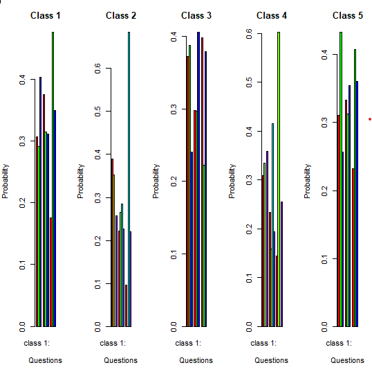
The visualization of item-response probabilities provides a comprehensive overview of the response patterns within each latent class, allowing for deeper insights into the underlying structure of the data analyzed using latent class analysis.
Conclusion
Latent Class Analysis (LCA) is a great method for finding hidden subgroups within data. Using the poLCA package in R, we can identify these subgroups, check how well our model fits the data, understand the characteristics of each subgroup, and visualize the results. By uncovering these hidden structures, LCA helps us to make better decisions in research and practice, such as targeting specific interventions, customizing marketing strategies, or gaining new insights about different groups in our population.
