The real estate market is a dynamic and complex sector that requires detailed analysis and insightful visualizations to understand trends and make informed decisions. A well-designed dashboard can comprehensively view market conditions, price trends, inventory levels, and other important metrics.
Project Overview
In this project, we’ll create a Real Estate Market Trends Dashboard using R. This dashboard will visualize key metrics such as median home prices, inventory levels, days on market, price per square foot, and sales volume. We will also demonstrate how to build an interactive dashboard using the Shiny package, allowing users to explore the real estate data dynamically.
Installing and Loading Necessary Libraries
Before starting, we will install and load the required libraries. R provides a rich set of libraries for data manipulation and visualization, such as shiny for interactive web applications, ggplot2 for plotting, and dplyr for data manipulation
install.packages(c("ggplot2", "shiny", "dplyr", "scales"))
Creating the Dashboard in R
Below are examples of how to create various components of a real estate market trends dashboard using R.
1. Median Home Prices
We will create a line chart to show the Median Home Prices.
library(ggplot2)

data <- data.frame(
  Month = as.Date(c('2023-01-01', '2023-02-01', '2023-03-01', '2023-04-01',
                    '2023-05-01')),
  MedianPrice = c(300000, 310000, 320000, 315000, 330000)
)

ggplot(data, aes(x = Month, y = MedianPrice)) +
  geom_line(color = 'blue') +
  geom_point(color = 'red') +
  labs(title = "Median Home Prices Over Time", x = "Month", y = "Median Price (USD)") +
  theme_minimal()
Output:
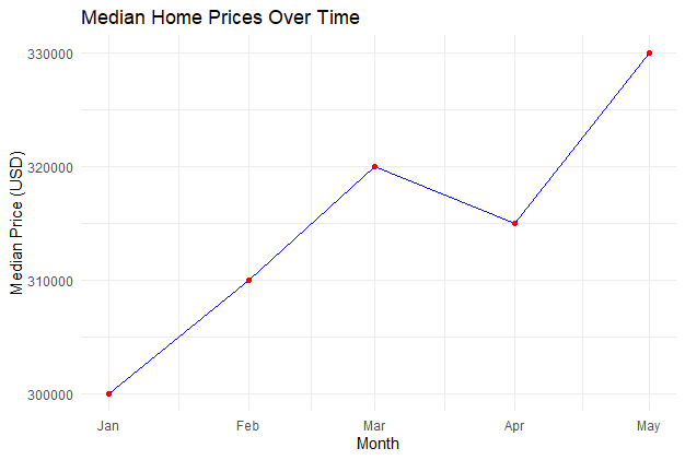
This line chart shows the trend of median home prices over time, helping stakeholders understand how prices are changing month to month.
2. Inventory Levels
Inventory management is a crucial aspect of supply chain and business operations. Proper management of inventory levels ensures that a company can meet customer demand without overstocking, which ties up capital, or understocking, which leads to missed sales opportunities.
data <- data.frame(
  Month = as.Date(c('2023-01-01', '2023-02-01', '2023-03-01', '2023-04-01',
                    '2023-05-01')),
  Inventory = c(1500, 1450, 1600, 1580, 1700)
)

ggplot(data, aes(x = Month, y = Inventory)) +
  geom_bar(stat = "identity", fill = 'skyblue') +
  labs(title = "Inventory Levels Over Time", x = "Month",
       y = "Number of Homes Available") +
  theme_minimal()
Output:
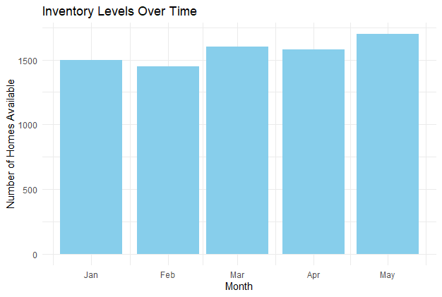
This bar chart visualizes the number of homes available for sale over time, providing insights into inventory trends.
3. Days on Market (DOM)
Days on Market (DOM) is a critical metric in real estate that measures the number of days a property has been listed for sale before it is sold.
data <- data.frame(
  Month = as.Date(c('2023-01-01', '2023-02-01', '2023-03-01', '2023-04-01', '2023-05-01')),
  DOM = c(30, 28, 35, 32, 31)
)

ggplot(data, aes(x = Month, y = DOM)) +
  geom_line(color = 'green') +
  geom_point(color = 'orange') +
  labs(title = "Average Days on Market Over Time", x = "Month", y = "Days on Market") +
  theme_minimal()
Output:
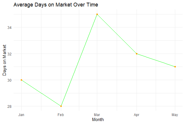
This line chart shows the average number of days properties remain on the market before being sold, indicating the speed of sales.
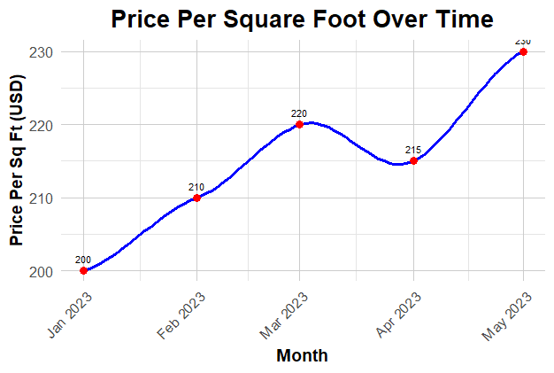
4. Price Per Square Foot
Price per square foot is a commonly used metric in real estate to evaluate the cost of a property relative to its size. This metric helps buyers, sellers, and investors understand the value of a property and make informed decisions
library(ggplot2)
library(scales)

data <- data.frame(
  Month = as.Date(c('2023-01-01', '2023-02-01', '2023-03-01', '2023-04-01',
                    '2023-05-01')),
  PricePerSqFt = c(200, 210, 220, 215, 230)
)

ggplot(data, aes(x = Month, y = PricePerSqFt)) +
  geom_smooth(method = "loess", se = FALSE, color = 'blue', size = 1.2) +
  geom_point(color = 'red', size = 3) +
  geom_text(aes(label = PricePerSqFt), vjust = -1, color = 'black', size = 3) +
  labs(
    title = "Price Per Square Foot Over Time",
    x = "Month",
    y = "Price Per Sq Ft (USD)"
  ) +
  scale_x_date(date_labels = "%b %Y", date_breaks = "1 month") +
  theme_minimal(base_size = 15) +
  theme(
    plot.title = element_text(hjust = 0.5, face = "bold", size = 20),
    axis.title.x = element_text(face = "bold", size = 14),
    axis.title.y = element_text(face = "bold", size = 14),
    axis.text.x = element_text(angle = 45, hjust = 1, size = 12),
    axis.text.y = element_text(size = 12),
    panel.grid.major = element_line(color = "grey80"),
    panel.grid.minor = element_line(color = "grey90")
  )
Output:
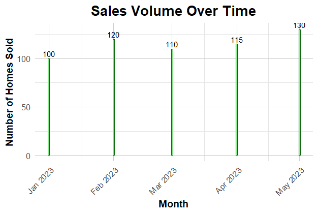
5. Sales Volume
To make the sales volume plot we can add enhancements such as customizing the color palette, adding data labels, adjusting the theme for better readability, and incorporating a smoother visual design. Here's an improved version of the plot.
library(ggplot2)
library(scales)

data <- data.frame(
  Month = as.Date(c('2023-01-01', '2023-02-01', '2023-03-01', '2023-04-01',
                    '2023-05-01')),
  SalesVolume = c(100, 120, 110, 115, 130)
)

ggplot(data, aes(x = Month, y = SalesVolume)) +
  geom_bar(stat = "identity", fill = 'lightgreen', color = 'darkgreen', width = 0.7) +
  geom_text(aes(label = SalesVolume), vjust = -0.3, color = 'black', size = 4) +
  labs(
    title = "Sales Volume Over Time",
    x = "Month",
    y = "Number of Homes Sold"
  ) +
  scale_x_date(date_labels = "%b %Y", date_breaks = "1 month") +
  theme_minimal(base_size = 15) +
  theme(
    plot.title = element_text(hjust = 0.5, face = "bold", size = 20),
    axis.title.x = element_text(face = "bold", size = 14),
    axis.title.y = element_text(face = "bold", size = 14),
    axis.text.x = element_text(angle = 45, hjust = 1, size = 12),
    axis.text.y = element_text(size = 12),
    panel.grid.major = element_line(color = "grey80"),
    panel.grid.minor = element_line(color = "grey90")
  )
Output:
6. Interactive Dashboard with Shiny
To create an interactive dashboard, we can use the shiny package. Here’s a basic example.
library(shiny)
library(ggplot2)

data <- data.frame(
  Month = as.Date(c('2023-01-01', '2023-02-01', '2023-03-01', '2023-04-01',
                    '2023-05-01')),
  MedianPrice = c(300000, 310000, 320000, 315000, 330000),
  Inventory = c(1500, 1450, 1600, 1580, 1700),
  DOM = c(30, 28, 35, 32, 31),
  PricePerSqFt = c(200, 210, 220, 215, 230),
  SalesVolume = c(100, 120, 110, 115, 130)
)
# UI
ui <- fluidPage(
  titlePanel("Real Estate Market Trends Dashboard"),
  sidebarLayout(
    sidebarPanel(
      selectInput("metric", "Choose a metric:",
                  choices = c("MedianPrice", "Inventory", "DOM", "PricePerSqFt",
                              "SalesVolume"))
    ),
    mainPanel(
      plotOutput("trendPlot")
    )
  )
)
# Server
server <- function(input, output) {
  output$trendPlot <- renderPlot({
    ggplot(data, aes_string(x = "Month", y = input$metric)) +
      geom_line(color = 'blue') +
      geom_point(color = 'red') +
      labs(title = paste(input$metric, "Over Time"), x = "Month", y = input$metric) +
      theme_minimal()
  })
}

shinyApp(ui = ui, server = server)
Output:
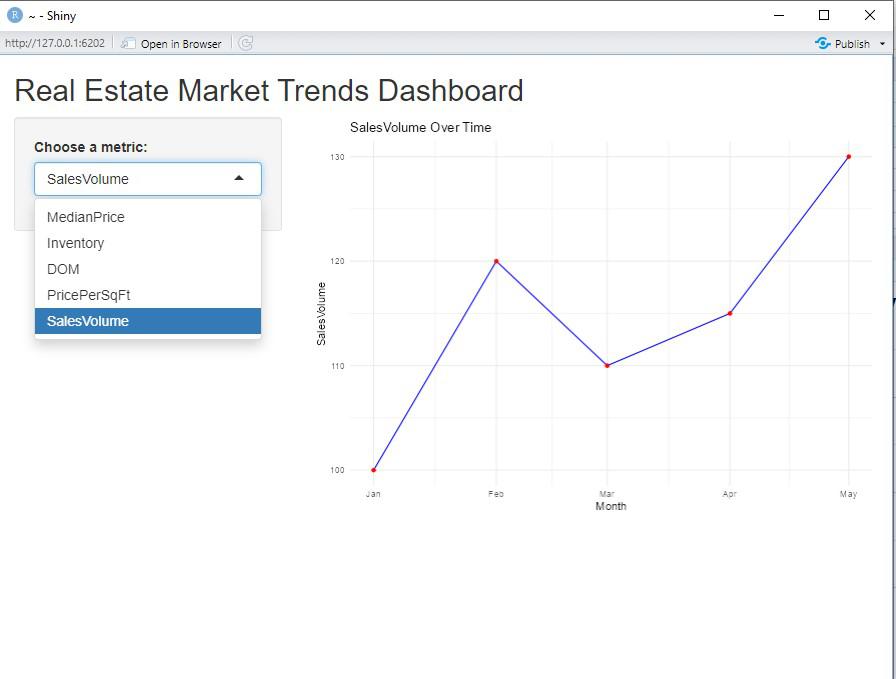
This shiny app allows users to interactively choose a metric to visualize. The line chart updates based on the selected metric, providing a flexible and dynamic view of the data.
Conclusion
From our dashboard, we can get:
- Key Insights: The dashboard visualizes critical metrics like median home prices, inventory levels, days on market, price per square foot, and sales volume.
- Dynamic Visualization: Using R and Shiny, the dashboard enables interactive exploration of data, helping stakeholders identify trends and changes over time.
- Informed Decision-Making: By analyzing these metrics, the dashboard assists in optimizing pricing strategies, making better investment decisions, and understanding overall market dynamics.
