Reduced Row Echelon Form (rref) Matrix in MATLAB

Reduced Row Echelon Form of a matrix is used to find the rank of a matrix and further allows to solve a system of linear equations. A matrix is in Row Echelon form if

• All rows consisting of only zeroes are at the bottom.
• The first nonzero element of a nonzero row is always strictly to the right of the first nonzero element of the row above it.

Example :

\left[ \begin{array}{ccccc} 1 & a_0 & a_1 & a_2 & a_3 \\ 0 & 0 & 2 & a_4 & a_5 \\ 0 & 0 & 0 & 1 & a_6\\ 0 & 0 & 0 & 0 & 0 \end{array} \right]

A matrix can have several row echelon forms. A matrix is in Reduced Row Echelon Form if

• It is in row echelon form.
• The first nonzero element in each nonzero row is a 1.
• Each column containing a nonzero as 1 has zeros in all its other entries.

Example:

{\displaystyle \left[{\begin{array}{ccccc}1&0&a_{1}&0&b_{1}\\0&1&a_{2}&0&b_{2}\\0&0&0&1&b_{3}\end{array}}\right]}

Where a1,a2,b1,b2,b3 are nonzero elements.

A matrix has a unique Reduced row echelon form. Matlab allows users to find Reduced Row Echelon Form using rref() method. Different syntax of rref() are:

• R = rref(A)
• [R,p] = rref(A)

Let us discuss the above syntaxes in detail:

rref(A)

It returns the Reduced Row Echelon Form of the matrix A using the Gauss-Jordan method.

% creating a matrix using magic(n)
% generates n*n matrix with values
% from 1 to n^2 where every row sum
% is equal to every column sum
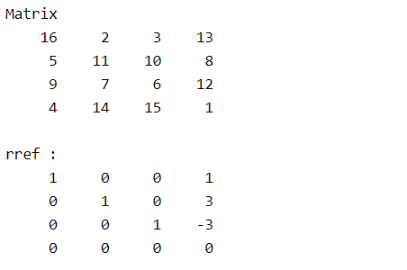
A = magic(4);
disp("Matrix");
disp(A);

% Reduced Row Echelon Form of A
RA = rref(A);
disp("rref :");
disp(RA);

Output :

rref(A)

• It returns Reduced Row Echelon Form R and a vector of pivots p
• p is a vector of row numbers that has a nonzero element in its Reduced Row Echelon Form.
• The rank of matrix A is length(p).
• R(1:length(p),1:length(p)) (First length(p) rows and length(p) columns in R) is an identity matrix.

% creating a matrix using magic(n)
% generates n*n matrix with values 
% from 1 to n^2 where every row sum
% is equal to every column sum
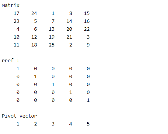
A = magic(5);
disp("Matrix");
disp(A);

% Reduced Row Echelon Form of A
[RA,p] = rref(A);
disp("rref :");
disp(RA);

% Displaying pivot vector p
disp("Pivot vector");
disp(p);

Output :

Finding solutions to a system of linear equations using Reduced Row Echelon Form:

The System of linear equations is  x+y+z=6\\ x+2y+3z=14\\ x+4y+7z=30

Coefficient matrix A is   \left[ \begin{array}{ccccc} 1 & 1 & 1 \\ 1 & 2 & 3\\ 1 & 4 & 7 \end{array} \right]

Constant matrix B is   \left[ \begin{array}{ccccc} 6 \\ 14\\ 30 \end{array} \right]

Then Augmented matrix [AB] is   \left[ \begin{array}{ccccc} 1 & 1 & 1 & 6\\ 1 & 2 & 3 & 14\\ 1 & 4 & 7 & 30 \end{array} \right]

% Coefficient matrix
A = [1  1  1;
     1  2  3;
     1  4  7];
     
% Constant matrix
b = [6 ;14; 30];

% Augmented matrix
M = [A b];
disp("Augmented matrix");
disp(M)

% Reduced Row echelon form of 
% Augmented matrix
R = rref(M);
disp("rref");
disp(R)

Output :

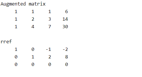
Then the reduced equations are x-z=-2\;, y+2z=8

It has infinite solutions, one can be x=1\;,y=2\;,z=3    .