Conditional formatting with custom formulas in Google Sheets allows you to apply dynamic formatting based on specific criteria that you define. This powerful feature enables you to highlight cells, rows, or ranges that meet particular conditions, making your data visually appealing and easier to analyze. In this guide, we'll walk you through the process of using custom formulas for conditional formatting in Google Sheets, helping you streamline your workflow and enhance data visualization.
Use a Custom Formula to Apply Conditional Formatting
Conditional formatting with custom formulas allows you to apply formatting rules based on specific conditions you define. Here's how to use it:
Step 1: Select the Range for Conditional Formatting
Select the Priority column (B2:B6) to highlight tasks with a "High" priority.

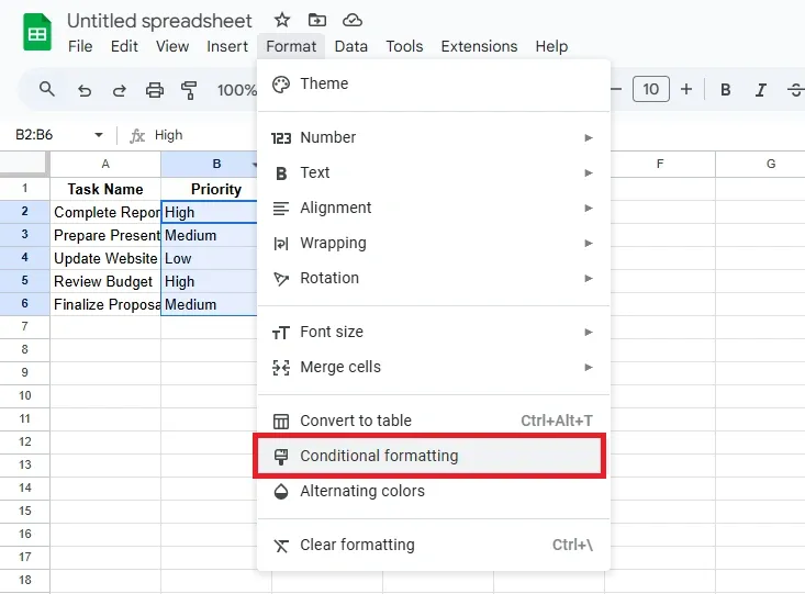
Step 2: Open the Conditional Formatting Menu
- Go to the Format menu at the top of Google Sheets.
- Select Conditional formatting from the dropdown menu. This will open the Conditional format rules panel on the right side.
Step 3: Choose "Custom Formula Is"
- In the Conditional format rules panel, click the dropdown under Format cells if.
- Select Custom formula is from the list.

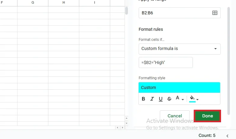
Step 4: Enter the Custom Formula
- To highlight tasks marked as "High" priority in column B:
- Enter the formula:
=$B2="High"This formula will highlight any cell in column B where the Priority is "High".

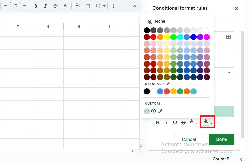
Step 5: Choose the Formatting Style
- Under Formatting style, click the paint bucket icon to choose the color or text style.
- Choose a background color (e.g., red) to highlight tasks with a "High" priority.
Step 6: Apply the Conditional Formatting
Click Done to apply the formatting rule to the selected range.
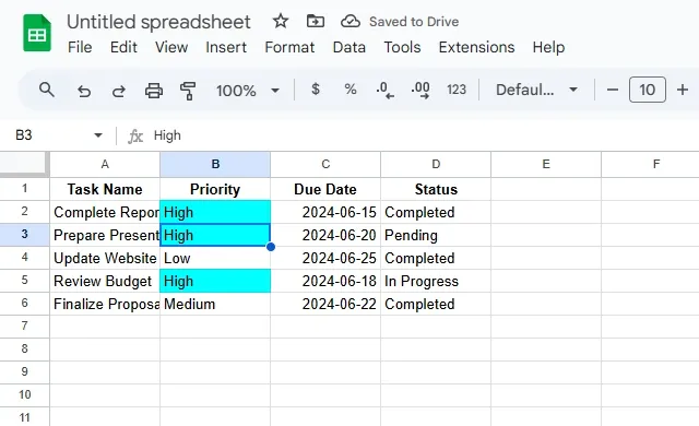
Step 7: Test the Formatting
- Enter different priorities in the Priority column (e.g., "Medium", "Low", etc.) and check if the cells with High priority get highlighted in red.
- Try changing the Priority for different rows and observe the conditional formatting being applied automatically based on the value.
Examples of Custom Formulas for Conditional Formatting in Google Sheets
Conditional formatting with custom formulas allows you to highlight data in unique ways based on specific conditions. Below are some examples:
| Formula | Purpose | Example |
|---|---|---|
=A1>100 | Highlights cells greater than 100 | Use this to identify values above a threshold. |
=A1="Complete" | Highlights cells with the exact text "Complete" | Useful for tracking task completion statuses. |
=ISBLANK(A1) | Highlights blank cells | Identify missing or incomplete data. |
=A1<TODAY() | Highlights dates before today | Ideal for overdue tasks or expired deadlines. |
=AND(A1>50, A1<100) | Highlights cells between 50 and 100 | Filter data within a specific range. |
=MOD(ROW(), 2)=0 | Highlights every other row | Use for alternating row colors for better readability. |
=$A1="Urgent" | Highlights entire rows where column A contains "Urgent" | Emphasize rows based on priority levels. |
=SEARCH("error", A1) | Highlights cells containing the word "error" | Use to flag issues or errors in data. |
=A1=A2 | Highlights duplicate values in consecutive rows | Useful for finding duplicates in sorted lists. |
=COUNTIF(A:A, A1)>1 | Highlights all duplicates in a column | Identify repeated entries across an entire column. |
=OR(A1="High", A1="Critical") | Highlights cells containing "High" or "Critical" | Great for marking important or critical items. |
=A1<>"" | Highlights non-empty cells | Differentiate populated cells from blank ones. |
These custom formulas allow for flexible and advanced conditional formatting to manage and visualize your data in Google Sheets.
Conclusion
Using conditional formatting with custom formulas in Google Sheets allows you to apply dynamic and flexible formatting rules based on specific conditions tailored to your needs. Whether you're highlighting high-priority tasks, flagging due dates, or organizing data based on complex criteria, custom formulas offer powerful control over how your data is visually represented. By following the steps outlined, you can enhance the readability and effectiveness of your spreadsheets, making them easier to analyze and more visually organized.
