


引言
首先,我们需要知道kalman滤波在卫星导航定位中主要是用来做做什么的。
Kalman 滤波在卫星定位中,用于在存在噪声和动态变化的情况下,将历元间的状态预测与卫星观测信息进行最优融合,从而连续、稳定地估计接收机位置及相关参数。
在 GNSS(如 GPS、北斗)卫星定位中,我们面临的首要问题是:卫星给出的观测值并不是完全准确的。观测过程中不可避免地会受到测量噪声、大气延迟、多路径效应以及接收机和卫星钟差等多种误差影响。而我们真正关心的,并不是这些带有误差的观测值本身,而是接收机的真实位置、钟差以及载波模糊度等状态参数。与此同时,定位并不是一次计算就结束的过程,卫星观测会以秒级不断更新,有些参数会随时间缓慢变化,比如接收机位置和钟差,而有些参数在一段时间内保持不变但事先未知,比如载波模糊度。问题的核心在于:每一历元的观测都存在误差,但我们又不能简单地丢弃历史信息,而只能依赖当前观测。
Kalman 滤波正是在这种背景下发挥作用的。可以把它理解成一个“边走边修正的定位管家”。在每一个历元,Kalman 滤波都会先根据上一时刻的估计结果和一定的运动模型,对当前状态进行预测。如果是静态站,它会认为接收机大概率仍然停留在原来的位置;如果是动态场景,它会根据已有的速度信息推测接收机向前移动了一段距离。这一步得到的是一个不依赖当前卫星观测的预测结果,但 Kalman 滤波也清楚,这种预测本身并不完全可靠。
当新的卫星观测到来之后,Kalman 滤波会利用这些观测对预测结果进行修正。卫星观测可以提供当前位置的线索,但同时又伴随着噪声。Kalman 滤波的关键思想就在于,根据预测结果和观测结果各自的不确定度,对两者进行加权融合。如果当前观测质量较好,就更偏向相信卫星信息;如果观测噪声较大,就更依赖之前的预测。通过这种方式,Kalman 滤波能够在每一个历元给出当前最可信的位置和相关参数估计。
Kalman滤波数学原理
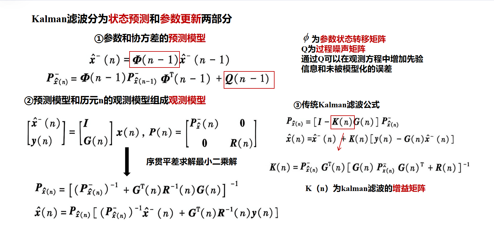
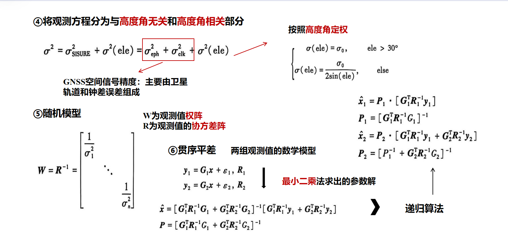
序贯平差求解最小二乘解
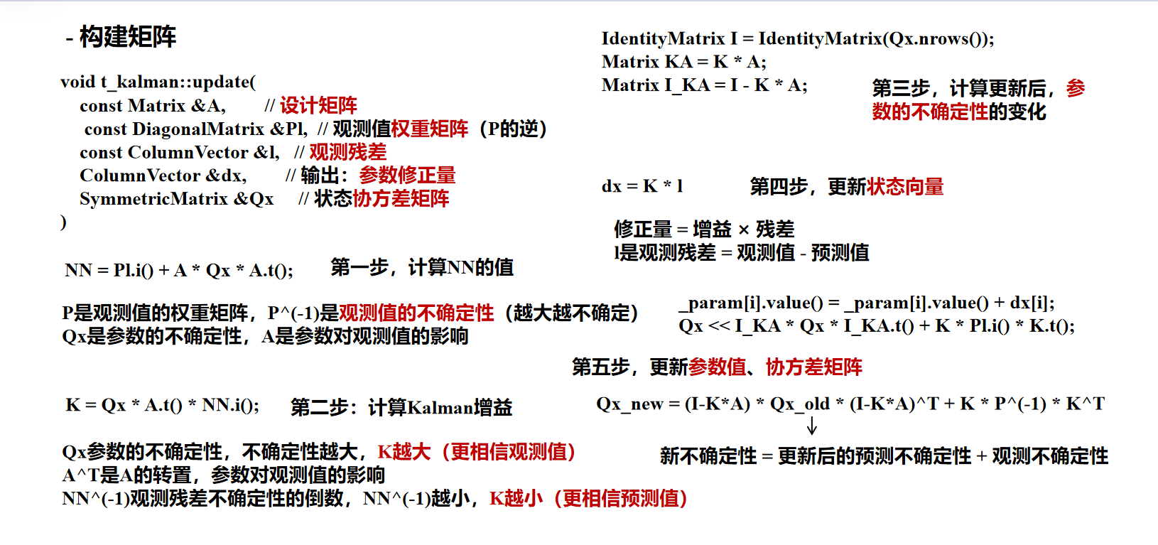
Kalman滤波实现
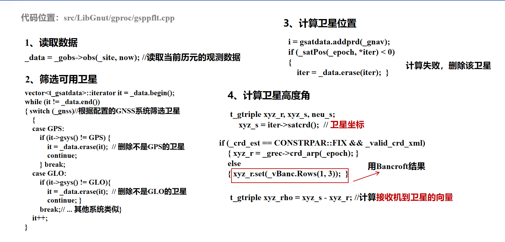
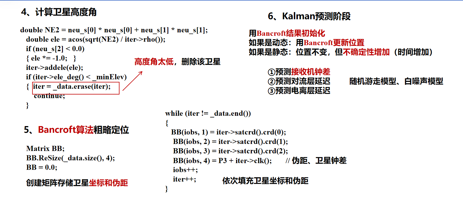
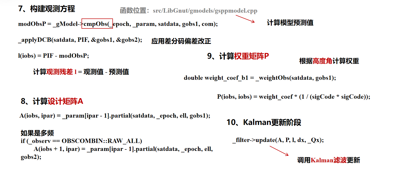
PPP实现流程
这部分将以武大的的GREAT-PVT中的代码为例,进行了简单的分析
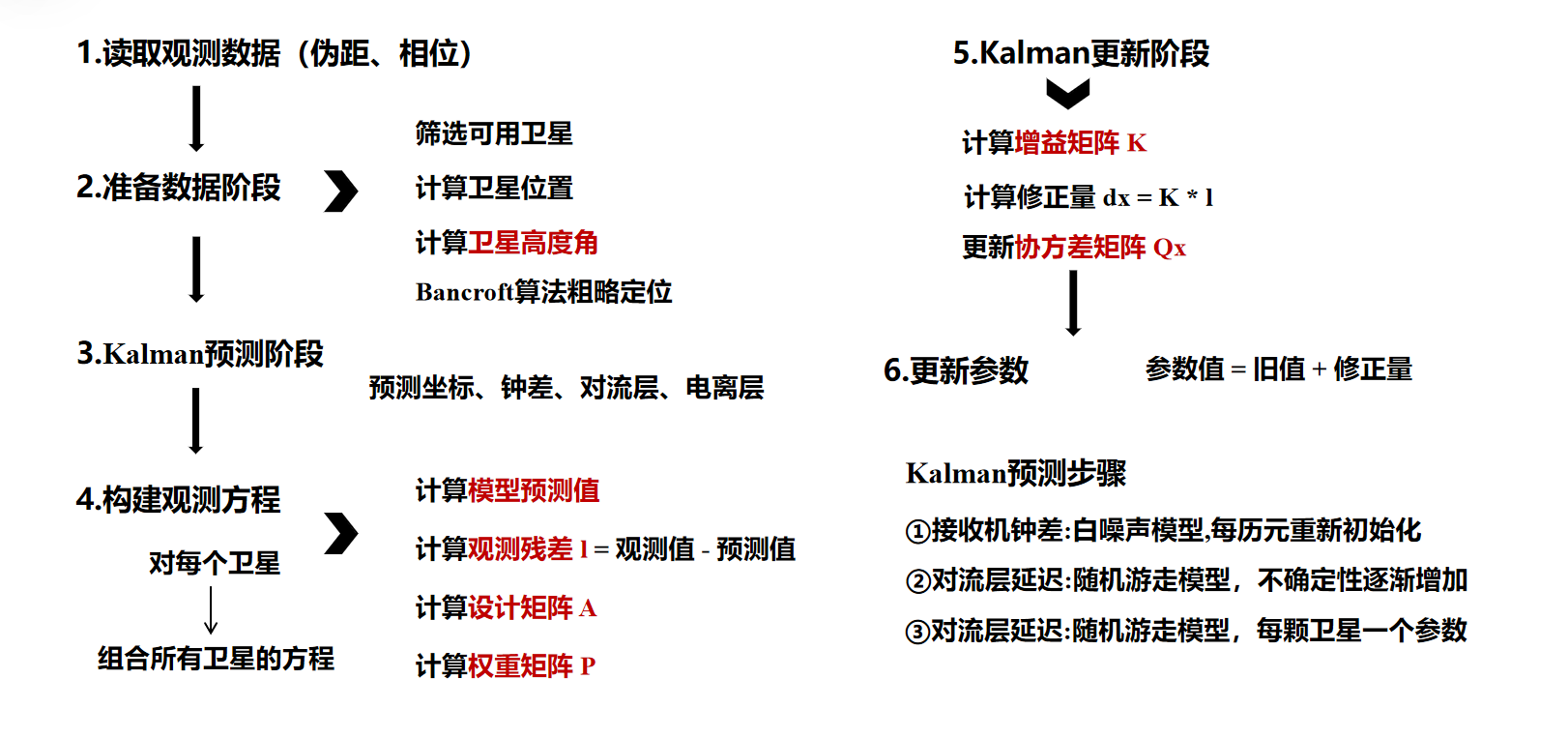
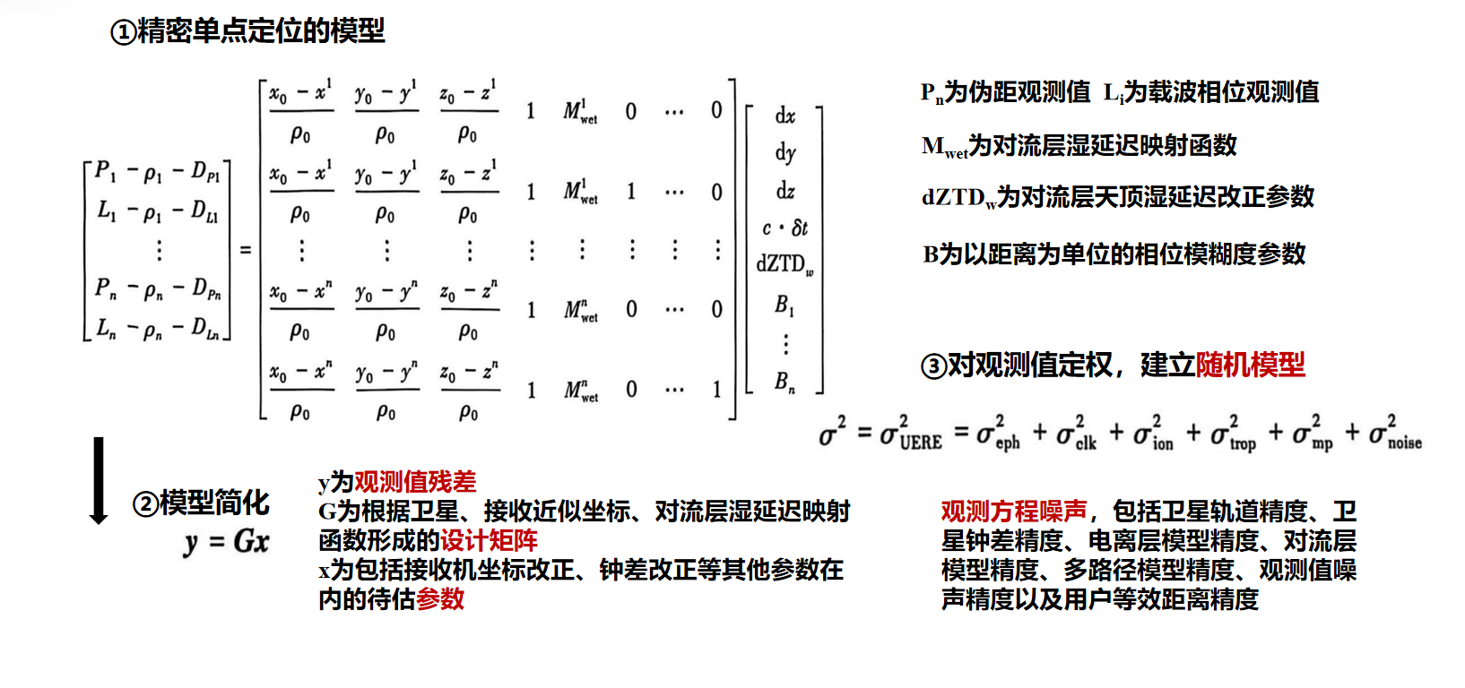
PPP实现
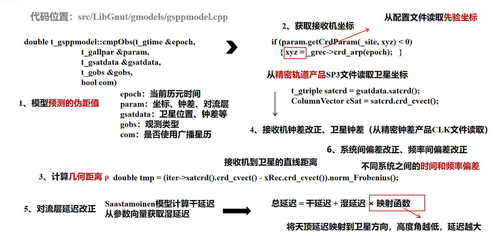
模型预测
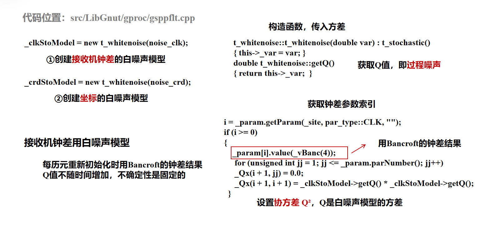
白噪声模型
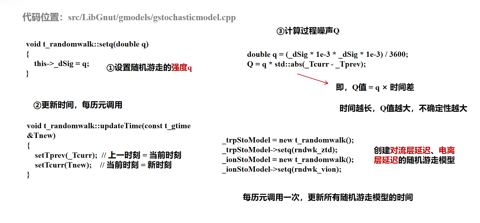
随机游走模型
代码示例
参考了深入浅出理解卡尔曼滤波【实例、公式、代码和图】中所给的kalman滤波的代码,为了适配本地,只做了微小的改动,原文将Kalman滤波的数学原理讲解得十分清晰
代码
# -*- coding: utf-8 -*-
"""
完整的卡尔曼滤波实现
对理想的一维匀加速直线运动模型,配有不精确的IMU和不精确的GPS,进行位置和速度观测
使用矩阵形式的卡尔曼滤波,同时估计位置和速度
"""
import numpy as np
import matplotlib.pyplot as plt
from matplotlib import font_manager
import warnings
import os
# ==================== 参数设置 ====================
t = np.linspace(1, 100, 100) # 在1~100s内采样100次
u = 0.6 # 加速度值,匀加速直线运动模型
v0 = 5 # 初始速度
s0 = 0 # 初始位置
# 过程噪声的协方差矩阵(运动模型的不确定性)
Q = np.array([[1e1, 0],
[0, 1e1]])
# 观测噪声的协方差矩阵(传感器测量误差)
R = np.array([[1e4, 0],
[0, 1e4]])
size = t.shape[0] + 1
dims = 2 # 状态维度:[位置, 速度]
# ==================== 卡尔曼滤波初始化 ====================
# 初始状态估计 [位置, 速度]
X = np.array([[s0], [v0]])
# 先验误差协方差矩阵的初始值
P = np.array([[0.1, 0],
[0, 0.1]])
# 状态转移矩阵(描述状态如何随时间变化)
F = np.array([[1, 1], # 位置 = 位置 + 速度*1
[0, 1]]) # 速度 = 速度(假设匀速,加速度通过控制项加入)
# 控制矩阵(描述控制输入如何影响状态)
B = np.array([[1 / 2], # 位置变化 = 0.5 * a * t^2,这里t=1
[1]]) # 速度变化 = a * t,这里t=1
# 观测矩阵(描述如何从状态得到观测值)
H = np.array([[1, 0], # 观测位置 = 状态位置
[0, 1]]) # 观测速度 = 状态速度
# ==================== 数据存储 ====================
# 真实值(仅用于模拟和对比,实际应用中不可知)
X_true = np.array([[s0], [v0]])
real_positions = np.zeros(size)
real_speeds = np.zeros(size)
real_positions[0] = s0
real_speeds[0] = v0
# 测量值(模拟传感器数据,实际应用中从GPS和IMU获取)
measure_positions = np.zeros(size)
measure_speeds = np.zeros(size)
measure_positions[0] = real_positions[0] + np.random.normal(0, R[0][0] ** 0.5)
measure_speeds[0] = real_speeds[0] + np.random.normal(0, R[1][1] ** 0.5)
# 卡尔曼滤波估计值(最优估计)
optim_positions = np.zeros(size)
optim_speeds = np.zeros(size)
optim_positions[0] = X[0][0]
optim_speeds[0] = X[1][0]
# 仅使用运动模型预测的值(不使用观测值修正,用于对比)
predict_positions = np.zeros(size)
predict_speeds = np.zeros(size)
predict_positions[0] = measure_positions[0]
predict_speeds[0] = measure_speeds[0]
X_predict = np.array([[measure_positions[0]], [measure_speeds[0]]])
# ==================== 卡尔曼滤波主循环 ====================
for i in range(1, t.shape[0] + 1):
# ========== 生成真实值(仅用于模拟,实际应用中不需要) ==========
# 过程噪声(运动模型的不确定性)
w = np.array([[np.random.normal(0, Q[0][0] ** 0.5)],
[np.random.normal(0, Q[1][1] ** 0.5)]])
# 真实状态更新(实际应用中不可知)
X_true = F @ X_true + B * u + w
real_positions[i] = X_true[0][0]
real_speeds[i] = X_true[1][0]
# ========== 生成观测值(模拟传感器数据) ==========
# 观测噪声(传感器测量误差)
v = np.array([[np.random.normal(0, R[0][0] ** 0.5)],
[np.random.normal(0, R[1][1] ** 0.5)]])
# 观测值 = 观测矩阵 * 真实状态 + 观测噪声
Z = H @ X_true + v
measure_positions[i] = Z[0][0]
measure_speeds[i] = Z[1][0]
# ========== 卡尔曼滤波:预测步骤 ==========
# 1. 状态预测:根据运动模型预测当前状态
X_pred = F @ X + B * u
# 2. 协方差预测:更新预测的不确定性
P_pred = F @ P @ F.T + Q
# ========== 卡尔曼滤波:更新步骤 ==========
# 3. 计算卡尔曼增益(权衡预测值和观测值的权重)
S = H @ P_pred @ H.T + R # 新息协方差
K = P_pred @ H.T @ np.linalg.inv(S) # 卡尔曼增益
# 4. 状态更新:结合预测值和观测值得到最优估计
X = X_pred + K @ (Z - H @ X_pred)
# 5. 协方差更新:更新估计的不确定性
P = (np.eye(2) - K @ H) @ P_pred
# ========== 仅使用运动模型预测(不使用观测值,用于对比) ==========
X_predict = F @ X_predict + B * u
# ========== 记录结果 ==========
optim_positions[i] = X[0][0]
optim_speeds[i] = X[1][0]
predict_positions[i] = X_predict[0][0]
predict_speeds[i] = X_predict[1][0]
# ==================== 可视化结果 ====================
t_plot = np.concatenate((np.array([0]), t))
plt.rcParams['font.family'] = 'sans-serif'
plt.rcParams['font.sans-serif'] = ['DejaVu Sans', 'Arial', 'Helvetica', 'sans-serif']
with warnings.catch_warnings():
warnings.filterwarnings('ignore', category=UserWarning)
warnings.filterwarnings('ignore', message='.*Glyph.*')
warnings.filterwarnings('ignore', message='.*missing from current font.*')
# 创建图像
fig = plt.figure(figsize=(14, 6))
# Position comparison plot
ax1 = plt.subplot(1, 2, 1)
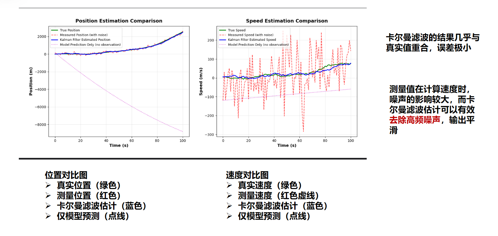
ax1.plot(t_plot, real_positions, 'g-', label='True Position', linewidth=2)
ax1.plot(t_plot, measure_positions, 'r--', label='Measured Position (with noise)', alpha=0.7)
ax1.plot(t_plot, optim_positions, 'b-', label='Kalman Filter Estimated Position', linewidth=2)
ax1.plot(t_plot, predict_positions, 'm:', label='Model Prediction Only (no observation)', alpha=0.7)
ax1.set_xlabel('Time (s)', fontsize=12, fontweight='bold')
ax1.set_ylabel('Position (m)', fontsize=12, fontweight='bold')
ax1.set_title('Position Estimation Comparison', fontsize=14, fontweight='bold', pad=10)
ax1.legend(loc='best', fontsize=9)
ax1.grid(True, alpha=0.3)
ax1.tick_params(labelsize=10)
# Speed comparison plot
ax2 = plt.subplot(1, 2, 2)
ax2.plot(t_plot, real_speeds, 'g-', label='True Speed', linewidth=2)
ax2.plot(t_plot, measure_speeds, 'r--', label='Measured Speed (with noise)', alpha=0.7)
ax2.plot(t_plot, optim_speeds, 'b-', label='Kalman Filter Estimated Speed', linewidth=2)
ax2.plot(t_plot, predict_speeds, 'm:', label='Model Prediction Only (no observation)', alpha=0.7)
ax2.set_xlabel('Time (s)', fontsize=12, fontweight='bold')
ax2.set_ylabel('Speed (m/s)', fontsize=12, fontweight='bold')
ax2.set_title('Speed Estimation Comparison', fontsize=14, fontweight='bold', pad=10)
ax2.legend(loc='best', fontsize=9)
ax2.grid(True, alpha=0.3)
ax2.tick_params(labelsize=10)
if ax1.get_xlabel() == '':
ax1.set_xlabel('Time (s)', fontsize=12, fontweight='bold')
if ax1.get_ylabel() == '':
ax1.set_ylabel('Position (m)', fontsize=12, fontweight='bold')
if ax2.get_xlabel() == '':
ax2.set_xlabel('Time (s)', fontsize=12, fontweight='bold')
if ax2.get_ylabel() == '':
ax2.set_ylabel('Speed (m/s)', fontsize=12, fontweight='bold')
plt.tight_layout(pad=3.0)
output_filename = 'kalman_filter_result.png'
try:
plt.savefig(output_filename, dpi=150, bbox_inches='tight', facecolor='white',
edgecolor='none', pad_inches=0.2)
print(f"\nImage successfully saved as: {output_filename}")
print(f" File path: {os.path.abspath(output_filename)}")
except Exception as e:
print(f"Error saving image: {e}")
try:
plt.show(block=False)
print("Image window opened (if environment supports)")
except Exception as e:
print(f"Warning: Cannot display image window (normal if running on server or no GUI environment)")
print(f" Image saved to file, please check: {output_filename}")
# ==================== 误差分析 ====================
# 计算均方根误差(RMSE)
position_rmse_measure = np.sqrt(np.mean((measure_positions - real_positions) ** 2))
position_rmse_kalman = np.sqrt(np.mean((optim_positions - real_positions) ** 2))
position_rmse_predict = np.sqrt(np.mean((predict_positions - real_positions) ** 2))
speed_rmse_measure = np.sqrt(np.mean((measure_speeds - real_speeds) ** 2))
speed_rmse_kalman = np.sqrt(np.mean((optim_speeds - real_speeds) ** 2))
speed_rmse_predict = np.sqrt(np.mean((predict_speeds - real_speeds) ** 2))
print("=" * 60)
print("Error Analysis (RMSE)")
print("=" * 60)
print(f"Position Error:")
print(f" Measured: {position_rmse_measure:.4f} m")
print(f" Kalman Filter: {position_rmse_kalman:.4f} m")
print(f" Model Prediction Only: {position_rmse_predict:.4f} m")
print(f" Improvement: {(1 - position_rmse_kalman / position_rmse_measure) * 100:.2f}%")
print()
print(f"Speed Error:")
print(f" Measured: {speed_rmse_measure:.4f} m/s")
print(f" Kalman Filter: {speed_rmse_kalman:.4f} m/s")
print(f" Model Prediction Only: {speed_rmse_predict:.4f} m/s")
print(f" Improvement: {(1 - speed_rmse_kalman / speed_rmse_measure) * 100:.2f}%")
print("=" * 60)
结果


 363
363

 被折叠的 条评论
为什么被折叠?
被折叠的 条评论
为什么被折叠?
 到【灌水乐园】发言


