Softmax回归——基于葡萄酒品类鉴别数据集

1．Softmax回归模型

相比于用于拟合问题的线性回归，Softmax回归则主要用于分类问题。对于待分类类别数为$q$，有$n$个样本，每个样本特征维度为$d$，则Softmax回归模型可表示为
$$o=Wx+b$$

$$\hat{y}=softmax(o)=\frac{\exp (o)}{\sum _{k=1}^q\exp (o_k)}$$
其中$x\in R^{d\times 1}$为单个样本特征，$W\in R^{q\times d}$为权重，$b\in R^{q\times 1}$为偏置，$\hat{y}\in R^{q\times 1}$为模型输出。样本真实标签$y\in R^{q\times 1}$为独热编码格式。

2. 基于最大似然的交叉熵损失公式推导

由于$\hat{y}$的值均在$(0,1)$范围内，可以利用均方误差作为损失函数进行模型训练。由于$sum(\hat{y})=1$，不能将误差$y-\hat{y}$假设为高斯分布的随机变量进行处理，因此利用均方误差作为损失函数不满足最大似然准则。

但也正是$sum(\hat{y})=1$，可以将$\hat{y}$假设为样本$x$属于各个类别的概率，此时可以利用最大似然准则推导出更合适的损失函数，推导过程如下：

首先定义条件概率$P(y^{(i)}|x^{(i)})$，表示模型输入第$i$个样本$x^{(i)}$，输出为真实样本标签$y^{(i)}$的概率。则
$$P(y^{(i)}|x^{(i)})=\sum _{j=1}^q{y}_j{\hat{y}}_j$$
对于样本集$\left\{X\in R^{n\times d},Y\in R^{n\times q}\right\}$，条件概率$P(Y|X)$表示为
$$P(Y|X)=\prod _{i=1}^{n}P(y^{(i)}|x^{(i)})$$
两边取对数
$$\begin{array}{rl}& \log P(Y|X)=\sum _{i=1}^n\log P(y^{(i)}|x^{(i)})=\sum _{i=1}^n\log \sum _{j=1}^q{y}_j{\hat{y}}_j\\ & =\sum _{i=1}^n\sum _{j=1}^q{y}_j\log {\hat{y}}_j=-\sum _{i=1}^{n}l(y^{(i)},x^{(i)})\end{array}$$
其中
$$l(y^{(i)},x^{(i)})=-\sum _{j=1}^q{y}_j\log {\hat{y}}_j$$
基于最大似然准则，$\sum _{i=1}^{n}l(y^{(i)},x^{(i)})$应取得最小值才能使得$P(Y|X)$最大，因此在假设Softmax输出为概率的条件下，基于最大似然准则推导的损失函数为
$$L(\hat{Y},Y)=\frac{1}{n}\sum _{i=1}^{n}l(y^{(i)},x^{(i)})$$
所推导出的函数$l(y,x)$被称为交叉熵函数，其和熵的计算公式形式很类似，因为是两个不同的概率分布，因此这里称为交叉熵。

《动手学深度学习》中有一段关于熵和交叉熵物理意义很形象的解释，这里引用如下：

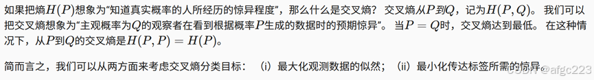
书中还给出了交叉熵函数的进一步推导及其导数计算公式：

3. Softmax回归与对数几率回归

1）对数几率回归采用sigmod函数进行分类，同样是将输出假设为概率，因此同样可以利用最大似然准则推导出交叉熵损失函数，两者损失函数是一致的。

2）对数几率回归只能用于解决二分类问题，而Softmax回归则可以解决二分类和多分类问题，因此Softmax回归使用范围更广。

3）Sigmod回归可以认为是Softmax回归的简化版，二分类的Softmax回归的权重参数量是Sigmod回归的两倍，因此模型的表达能力要更强。

4. 基于葡萄酒品类鉴别数据集的仿真验证

所采用的数据集共有三个类别葡萄酒，包括酒精含量、苹果酸，色调等13种不同的特征，一共178个样本，将其中30%作为测试集。

设置epochs=200，学习率0.01，网络训练的Loss函数下降过程为

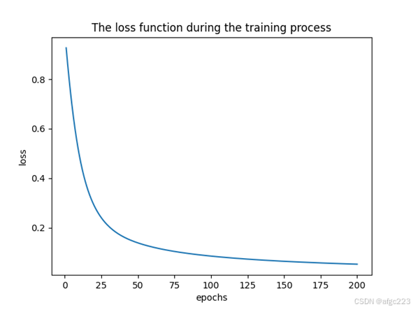
测试集54个样本的真实标签与模型输出标签的对比结果为

其中有一个测试样本出现错误，测试准确率为98.15%。

仿真代码如下：

import numpy as np
import torch
import torch.nn as nn
import torch.optim as optim
from sklearn import datasets
from sklearn.model_selection import train_test_split
from sklearn.preprocessing import StandardScaler
from sklearn.metrics import accuracy_score
import matplotlib.pyplot as plt

# Step 1: 加载 Wine 数据集
wine = datasets.load_wine()
X = wine.data
y = wine.target

# Step 2: 数据预处理（标准化）
scaler = StandardScaler()
X = scaler.fit_transform(X)

# Step 3: 将数据集分为训练集和测试集
X_train, X_test, y_train, y_test = train_test_split(X, y, test_size=0.3, random_state=42)

# Step 4: 将 NumPy 数组转换为 PyTorch 张量
X=torch.tensor(X, dtype=torch.float32)
y=torch.tensor(y, dtype=torch.long)
X_train_tensor = torch.tensor(X_train, dtype=torch.float32)
X_test_tensor = torch.tensor(X_test, dtype=torch.float32)
y_train_tensor = torch.tensor(y_train, dtype=torch.long)
y_test_tensor = torch.tensor(y_test, dtype=torch.long)

# Step 5: 定义 Softmax 回归模型
class SoftmaxRegression(nn.Module):
    def __init__(self, input_dim, output_dim):
        super(SoftmaxRegression, self).__init__()
        self.linear = nn.Linear(input_dim, output_dim)
    
    def forward(self, x):
        return self.linear(x)

# 创建模型实例
model = SoftmaxRegression(input_dim=X_train.shape[1], output_dim=3)  # 3 是葡萄酒的类别数

# Step 6: 定义损失函数和优化器
criterion = nn.CrossEntropyLoss()  # 交叉熵损失函数（适用于多分类问题）
optimizer = optim.Adam(model.parameters(), lr=0.01)  # Adam 优化器

# Step 7: 训练模型
num_epochs = 200
L_all=np.zeros(num_epochs)
for epoch in range(num_epochs):
    # 前向传播
    outputs = model(X_train_tensor)
    loss = criterion(outputs, y_train_tensor)
    
    # 反向传播和优化
    optimizer.zero_grad()  # 清零梯度
    loss.backward()  # 计算梯度
    optimizer.step()  # 更新权重
    L_all[epoch] = criterion(model(X), y).item()
    if (epoch+1) % 10 == 0:
        print(f'Epoch [{epoch+1}/{num_epochs}], Loss: {loss.item():.4f}')

# Step 8: 评估模型
with torch.no_grad():  # 不计算梯度，节省内存
    # 对测试集进行预测
    outputs = model(X_test_tensor)
    _, predicted = torch.max(outputs, 1)
    
    # 计算准确率
    accuracy = accuracy_score(y_test_tensor.numpy(), predicted.numpy())
    print(f'Accuracy on test set: {accuracy * 100:.2f}%')

# 可视化训练Loss函数
plt.plot(np.arange(num_epochs)+1,L_all)
plt.title('The loss function during the training process')
plt.xlabel('epochs')
plt.ylabel('loss')
plt.show()

# 可视化预测结果
plt.scatter(np.arange(len(X_test_tensor))+1,y_test_tensor.numpy(),color='blue',label='True',marker='s')
plt.scatter(np.arange(len(X_test_tensor))+1, predicted.numpy(),color='red',label='pred')
plt.xlabel('index')
plt.ylabel('MPG')
plt.title('True vs Predicted MPG')
plt.legend()
plt.show()  

5．参考

《动手学深度学——Pytorch版》，阿斯顿张，李沐等著，p71-p73