


 本文详细介绍了如何使用Matplotlib进行折线图、柱状图、饼图和直方图的绘制,包括颜色、线条样式等属性设置,以及坐标轴标签、范围、刻度调整和美化技巧。此外,还展示了如何设置图例、标题、网格和多图效果,以及高级图表如散点图、热图和三维图形的制作。
Matplotlib数据可视化
1. 通过Matplotlib绘制各种图形
1.1 绘制折线图
from matplotlib import pyplot as plt	# import matplotlib.pyplot as plt
import matplotlib
import numpy as np
# 通过Numpy设置x轴和y轴
x = np.arange(1, 6, 1)	# 利用arange方法创建1~5的数列
y = np.array([5, 15, 9, 16, 18])
# 通过plot方法绘制折线
plt.plot(x, y)
plt.show()

1.2 绘图时的通用属性参数
| 属性名 | 含义 |
|---|---|
| color | 线条的颜色 |
| linewidth | 线条的宽度 |
| linestyle | 线条的样式 |
| marker | 标记方式 |
| alpha | 透明度,取值从0到1,值越小越透明 |
import matplotlib.pyplot as plt
import matplotlib
import numpy as np
# 通过Numpy设置x和y轴的坐标
x = np.arange(5)
plt.plot(x, x*0.5, color = '#ff0011', linewidth = '5', linestyle = ':', alpha = 0.5)
plt.plot(x, x, color = 'red', linewidth = '2', linestyle = '--', marker = 'o')
plt.plot(x, x*1.5, color = 'blue', linewidth = '3', linestyle = '-.', marker = 'v')
plt.show()

1.3 绘制柱状图
在Matplotlib库中绘制柱状图(也叫条状图)的方法原型如下:
matplotlib.pyplot.bar(left, height, alpha = 1, width = 0.8, color = , edgecolor = , label = , lw = 3)。以下为参数详细说明:
| 参数 | 说明 |
|---|---|
| left | x轴的位置序列 |
| height | y轴的数值序列 |
| alpha | 透明度 |
| width | 柱形图的宽度(一般取值0.8) |
| color | 柱形图的填充色 |
| edgecolor | 柱形图的边缘颜色 |
| label | 用来设置图例 |
| lw | 线的宽度 |
# coding = utf-8
import matplotlib.pyplot as plt

# x轴刻度
x = [1, 2, 3, 4]
# y轴刻度
y = [80, 70, 75, 110]
width = [0.2, 0.4, 0.6, 0.8]
color = ['red', 'yellow', 'blue', 'green']
x_label = ['class_1', 'class_2', 'class_3', 'class_4']
# 绘制x刻度标签
plt.xticks(x, x_label)
# 绘制柱状图
plt.bar(x, y, color = color, width = width)
plt.show()

1.4 绘制饼图
在统计学中,饼图通常以二维或者三维的形式直观的展示统计数据中的每一项相对于总数的大小。在Matplotlib中,我们通过pyplot.pie方法来绘制二维饼图,方法使用的相关参数如下所示。
| 参数 | 含义 |
|---|---|
| label | 该饼图的说明文字 |
| sizes | 每个统计项的数字 |
| explode | 该块饼图离开中心点的位置 |
| radius | 半径,默认为1 |
| colors | 每块饼图的颜色 |
| startangle | 起始角度,默认图是从X轴正方向逆时针画起,比如设置为45,则表示从X轴逆时针方向45度开始画起 |
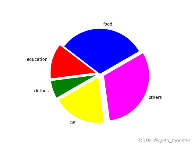
"""coding = utf-8"""
import matplotlib.pyplot as plt
items = ['food', 'education', 'clothes', 'car', 'others']
sizes = [5000, 2000, 1000, 3000, 5000]
explode = (0, 0.1, 0.1, 0.1, 0.1)
colors = ['blue', 'red', 'green', 'yellow', '#ff00ff']
plt.pie(sizes, explode = explode, labels = items, startangle = 30, colors = colors)
plt.show()
1.5 绘制直方图
虽然柱状图和直方图都是由若干个柱形区域组成,但是从统计意义上来看它们的含义是不同的。柱状图可以用来表现每个分类的数值,例如每个班级的平均分;直方图用来展现每个区域的分布情况,例如用来统计某次考试中0~100分每个区间里有多少人。直方图还有一个特点就是没有间隔,而柱状图是有间隔的。
在直方图中,一般是使用X轴表示数据区间,Y轴表示该区间的数据分布情况,绘制方法原型如下所示,并给出了相关常用参数的说明。
pyplot.hist(x, bins = None, sensity = None, histtype = ‘bar’, align = ‘mid’, color = None, label = None)
| 参数 | 含义 |
|---|---|
| x | 对应X轴,最终的直方图将对数据集进行统计 |
| bins | 指定对应的柱状图的个数 |
| histtype | 直方图的形状,可选‘bar’、‘barstacked’、‘step’、‘stepfilled’,默认是bar,tep使用的是梯形状,stepfilled会对梯状内部进行填充 |
| align | 可选’left’、‘mid’或’right’,默认是’mid’,用来控制柱状图的水平分布,如果选left或right,就会有部分空白区域,推荐使用默认 |
| color | 直方图的颜色 |
| density | Bool类型,默认是False,表示展示频数统计结果,为True则展示频率统计结果 |
| label | 标签文字,展示图标时能用到 |
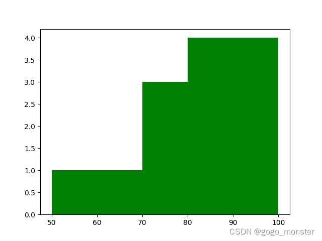
"""coding = utf-8"""
import matplotlib.pyplot as plt
import numpy as np
# 分数明细
x = [98, 87, 96, 82, 70, 65, 93, 72, 85, 58, 76, 92, 85]
# 设置连续的边界值,即直方图的分布区间,比如[50,60]等
bins = np.arange(50, 101, 10)
# 绘制直方图,统计各个区间的数值
plt.hist(x, bins, color = 'green')
plt.show()
2. 设置坐标技巧
2.1 设置X和Y坐标标签并展示中文
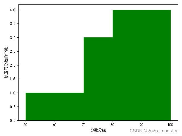
"""coding = utf-8"""
import matplotlib.pyplot as plt
import numpy as np
# 分数明细
x = [98, 87, 96, 82, 70, 65, 93, 72, 85, 58, 76, 92, 85]
# 设置连续的边界值,即直方图的分布区间,比如[50,60]等
bins = np.arange(50, 101, 10)
# 绘制直方图,统计各个区间的数值
plt.hist(x, bins, color = 'green')

# 设置中文
plt.rcParams['font.scans-serif'] = ['SimHei']
plt.xlabel('分数分组')
plt.ylabel('该区间分数的个数')
plt.show()
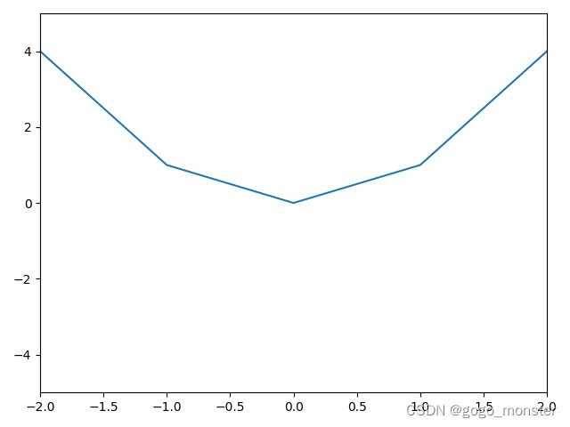
2.2 设置坐标范围
可以通过设置xlim和ylim方法设置X轴和Y轴的展示范围。
"""coding = utf-8"""
import matplotlib.pyplot as plt
import numpy as np
x = np.arange(-10, 11, 1)
plt.plot(x, x**2)
plt.xlim(-2, 2)
plt.ylim(-5, 5)
plt.show()
2.3 设置坐标的主刻度和次刻度
如果坐标轴上刻度文字显示过密,效果就会很不美观,此时可以设置主次刻度。
"""coding = utf-8"""
import numpy as np
import matplotlib.pyplot as plt
from matplotlib.ticker import MultipleLocator, FormatStrFormatter

# 将X轴主刻度设置为2的倍数
xmajorLocator = MultipleLocator(2)
# 设置X轴标签的格式
xmajorFormatter = FormatStrFormatter('%1.1f')   # “%1.1f”表示带一位小数的浮点型格式
# 将X轴次刻度设置为0.5的倍数
xminorLocator = MultipleLocator(0.5)

# 将Y轴主刻度设置为0.2的倍数
ymajorLocator = MultipleLocator(0.2)
# 设置Y轴标签的格式
ymajorFormatter = FormatStrFormatter('%1.2f')   # “%1.2f”表示带两位小数的浮点型格式
# 将Y轴次刻度设置为0.1的倍数
yminorLocator = MultipleLocator(0.1)

x = np.arange(0, 10, 0.1)
# 设置子图,在ax里设置坐标轴刻度
ax = plt.subplot(111)
# 设置主刻度标签的位置、标签文本的格式
ax.xaxis.set_major_locator(xmajorLocator)
ax.xaxis.set_major_formatter(xmajorFormatter)
ax.yaxis.set_major_locator(ymajorLocator)
ax.yaxis.set_major_formatter(ymajorFormatter)

# 显示次刻度标签的位置
ax.xaxis.set_minor_locator(xminorLocator)
ax.yaxis.set_minor_locator(yminorLocator)
y = np.cos(x)   # 绘图
plt.plot(x, y)
plt.show()

2.4 设置并旋转坐标刻度文字
"""coding = utf-8"""
import numpy as np
import matplotlib.pyplot as plt
# 折线图
x = np.array([1, 2, 3, 4, 5])
y = np.array([21, 20.5, 21.6, 21.8, 22])
# rotation设置的值是标尺的旋转角度
plt.xticks(x, ('20200101', '20200105', '20200110', '20200115', '20201020'), rotation = 30)
plt.yticks(np.arange(20, 22.5, 0.2), rotation = 30)
plt.ylim(20, 22)

# 设置中文
plt.rcParams['font.sans-serif'] = ['SimHei']
plt.xlabel('日期')
plt.ylabel('收盘价')
plt.plot(x, y, color = 'red')
plt.show()

至此,关于坐标轴设置的若干技巧,总结如下:
- 在绘制折线图等图形时,依然要通过数字(而不是文字)来设置X轴和Y轴的坐标。
- 如果要展示指定范围的数据,可以通过xlim和ylim来指定坐标轴的展示范围。注意,这两个方法的参数也是数字,而不是文字。
- 可以通过xlabel和ylabel来定义坐标轴的标签文字,从而指定相关坐标轴是展示哪类数据的。
- 可以通过MultipleLocator方法设置主次刻度,也可以通过FormatStrFormatter方法设置坐标轴刻度上数字的展示格式。
- 若要在坐标轴刻度上展示文字,而不是数字坐标,则可以通过xticks或yticks方法用rotation参数来实现刻度文字的旋转效果。
3. 增加可视化美观效果
3.1 设置图例
为了让图表更易于理解,往往会添加图例,在之前绘制图形时所用的label参数就和图例有关,绘制图例的方法是plt.legend。
"""coding = utf-8"""
import numpy as np
import matplotlib.pyplot as plt

x = np.arange(-3, 4)
plt.xlim(-3,3)
plt.plot(x, x, color = "green", label = 'y = x')
plt.plot(x, 2*x, color = "red", label = 'y = 2x')
plt.plot(x, 3*x, color = "yellow", label = 'y = 3x')
plt.legend(loc = 'best')   # 绘制图例
plt.show()

loc参数值及展示位置的对应关系表:
| 数值参数值 | 字符串参数值 | 图例位置 |
|---|---|---|
| 0 | best | 最适合的位置 |
| 1 | upper right | 右上角 |
| 2 | upper left | 左上角 |
| 3 | lower left | 左下角 |
| 4 | lower right | 右下角 |
| 5 | right | 右侧 |
| 6 | center left | 左侧中间 |
| 7 | center right | 右侧中间 |
| 8 | lower center | 下侧中间 |
| 9 | upper center | 上侧中间 |
| 10 | center | 中间 |
3.2 设置中文标题
在绘制图表时,可以通过title方法设置图表的标题,该方法的常用参数如下:
- fontsize表示标题的字体大小,常用参数有xx-small、x-small、small、medium、large、x-large、和xx-large等,默认值为12。
- fontweight表示字体的粗细,常用参数有light、normal、medium、semibold、bold、heavy和black。
- fontstyle表示字体类型,常用参数有normal、italic和oblique。
- verticalalignment表示水平对齐方式,可用参数有center、top、bottom和baseline。
- horizontalalignment表示垂直对齐方式,可用参数有left、right和center。
"""coding = utf-8"""
import matplotlib.pyplot as plt

items = ["饮食", "教育", "衣服", "汽车花费", "其他"]
sizes = [5000, 2000, 1000, 3000, 1000]
explode = (0, 0.1, 0.1, 0.1, 0.1)
colors = ["red", "yellow", "blue", "green", "purple"]
plt.pie(sizes, explode = explode, labels = items, startangle = 30, colors = colors)
plt.rcParams["font.sans-serif"] = ["SimHei"]    # 设置中文
# 设置标题
plt.title("本月开支", fontsize = "large", fontweight = 'bold', verticalalignment = 'center')
plt.show()

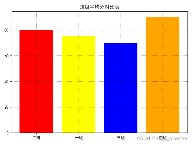
3.3 设置网格效果
如果能够在图表中添加横竖线式的网格效果,就可以让用户直观的横向或竖向的对比数据,通过Matplotlib库中的grid方法可以在图表中引用网格,其中同样可以通过传入参数指定颜色和线条类型等属性。
"""coding = utf-8"""
import matplotlib.pyplot as plt

x = [1, 2, 3, 4]    # X轴刻度
y = [80, 75, 70, 90]    # Y轴刻度
color = ['red', 'yellow', 'blue', 'orange']  # 设置每一列的颜色
x_label = {'一班', '二班', '三班', '四班'}
# 绘制X刻度标签
plt.xticks(x, x_label)
plt.rcParams['font.sans-serif'] = ['SimHei']    # 设置中文
# 设置标题
plt.title('班级平均分对比表')
# 绘制柱状图
plt.bar(x, y, color = color)
plt.grid(linewidth = '1', linestyle = ':', color = 'black', alpha = 0.5)
plt.show()
4. 设置多图和子图效果
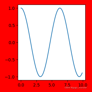
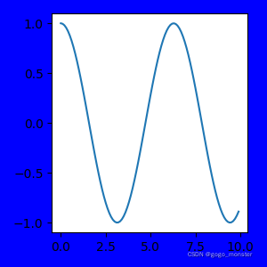
4.1 通过figure对象同时绘制多张图
在Matplotlib库中,通过figure对象可以绘制一块白板,设置白班的大小、边界颜色和背景演示等属性,下面给出该对象的构造方法。
figure(num = None, figsize = None, dpi = None, facecolor = None, edgecolor = None, frameon = True)
- num:表示当前图片的编号或名称
- figsize:表示宽度和高度,单位是英寸
- dpi:用来指定分辨率,即每英寸多少个像素,默认值为80
- facecolor:表示背景颜色
- edgecolor:表示边界颜色
- frameon:表示是否显示边框,默认值为True,也就是显示边框
"""coding = utf-8"""
import numpy as np
import matplotlib.pyplot as plt

x = np.arange(0, 10, 0.1)
# 第一个figure
plt.figure(num = 1, figsize = (3, 3), facecolor = 'red')
plt.plot(x, np.cos(x))

# 第二个figure
plt.figure(num = 2, figsize = (3, 3), facecolor = 'yellow')
plt.plot(x, np.cos(x))

# 第三个figure
plt.figure(num = 3, figsize = (3, 3), facecolor = 'blue')
plt.plot(x, np.cos(x))

# 图片展示
plt.show()
| 
| 
| 
|
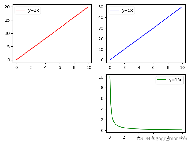
4.2 通过add_subplot方法绘制子图
以下给出示例演示通过figure的add_subplot方法绘制子图。
"""coding = utf-8"""

import numpy as np
import matplotlib.pyplot as plt

x = np.arange(0, 10, 0.1)
# 新建figure对象
fig = plt.figure()
# 子图1
ax1 = fig.add_subplot(2, 2, 1)
ax1.plot(x, 2*x, label = 'y=2x', color = 'red')
ax1.legend()

# 子图2
ax2 = fig.add_subplot(2, 2, 2)
ax2.plot(x, 5*x, label = 'y=5x', color = 'blue')
ax2.legend()

# 子图3
ax2 = fig.add_subplot(2, 2, 4)
ax2.plot(x, 1/x, label = 'y=1/x', color = 'green')
ax2.legend()

# 效果展示
plt.show()
4.3 通过subplot方法绘制子图
除了通过figure对象的add_subplot方法绘制子图外,还能通过pyplot对象的subplot方法来绘制子图。
"""coding = utf-8"""

import numpy as np
import matplotlib.pyplot as plt

x = np.arange(0, 10, 0.1)
plt.subplot(2, 1, 1)    # 第一个子图在2*1的第1个位置
plt.plot(x, 2*x)

plt.subplot(2, 2, 3)    # 第二个子图在2*2的第3个位置
plt.plot(x, 4*x)

plt.subplot(2, 2, 4)    # 第三个子图在2*2的第4个位置
plt.plot(x, 1/x)

# 效果展示
plt.show()

4.4 子图共享X轴坐标轴
在一些数据统计的场景中,若干个子图可以共享X轴。
"""coding = utf-8"""

import numpy as np
import matplotlib.pyplot as plt

# 分数明细
class1 = [98, 87, 96, 82, 70, 65, 93, 72, 85, 58, 76, 92, 85]
class2 = [87, 55, 92, 98, 95, 78, 72, 84, 96, 57, 87, 95, 95]
# 设置两个子图,并共享X轴
figure, (axClass1, axClass2) = plt.subplots(2, sharex = True, figsize = (10, 6))
# 设置连续的边界值,即直方图的分布区间,比如[50,60]等
bins = np.arange(50, 101, 10)
# 设置中文,并设置两个子图的标题
plt.rcParams['font.sans-serif'] = ['SimHei']
axClass1.set_title('一班的成绩分布图')
axClass2.set_title('二班的成绩分布图')
# 在两个子图里绘制直方图,统计各个区间的数值
axClass1.hist(class1, bins, color = 'red')
axClass2.hist(class2, bins, color = 'blue')
plt.show()

4.5 在大图中绘制子图
"""coding = utf-8"""

import numpy as np
import matplotlib.pyplot as plt
# 新建figure对象
fig = plt.figure()
ax = fig.add_axes([0.1, 0.1, 0.9, 0.9])
child_ax = fig.add_axes([0.7, 0.2, 0.2, 0.2])
x = np.arange(0, 10.1, 0.1)
ax.plot(x, np.sin(x), color = 'red')
# 子图
childX = np.arange(5, 6.1, 0.1)
child_ax.plot(childX, np.sin(childX), color = 'blue')
plt.show()

5. 绘制高级图表
5.1 绘制散点图
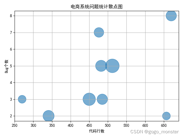
在散点图中,不仅能够展示数据点在直角坐标系平面上的分布,还能通过每个点的面积展示第三维信息。如下所示代码案例将展示某系统里模块的代码行数和bug数的关系,而且将用散点图的面积大小展示该模块里被Sonar扫描出来的违反代码规约现象的次数。
"""coding = utf-8"""

import numpy as np
import matplotlib.pyplot as plt

# 新建figure对象
fig, ax = plt.subplots()
codeLines = np.array([512, 341, 450, 270, 670, 482, 476, 657, 485])
codeBugs = np.array([5, 2, 3, 3, 8, 5, 7, 2, 3])
sonarWarnings = np.array([12, 8, 10, 4, 7, 8, 6, 4, 7])
ax.scatter(codeLines, codeBugs, s = sonarWarnings * 100, alpha = 0.6)
plt.rcParams['font.sans-serif'] = ['SimHei']    # 设置中文
# 设置标题
plt.title('电商系统问题统计散点图', fontsize = 'large', fontweight = 'bold')
plt.xlabel('代码行数')
plt.ylabel('Bug个数')
plt.grid()
plt.show()
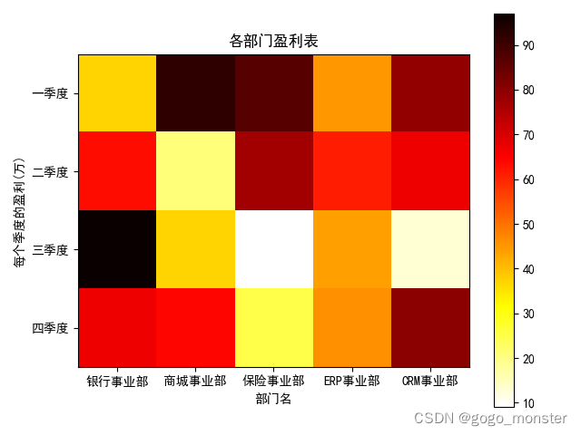
5.2 绘制热图
热图(heatmap)能够通过色差等方式展示不同样本数据间的差异,从而使报表数据更加直观、更易于理解。在matplotlib库中,可以通过imshow方法来绘制热图。
"""coding = utf-8"""

import matplotlib.pyplot as plt
xLabel = ['银行事业部', '商城事业部', '保险事业部', 'ERP事业部', 'CRM事业部']
yLabel = ['一季度', '二季度', '三季度', '四季度']
# 4个季度的盈利数据
data = [[37, 92, 87, 45, 79],
        [63, 21, 77, 61, 67],
        [97, 37, 9, 44, 13],
        [67, 64, 25, 46, 80]]
fig = plt.figure()
# 定义子图
ax = fig.add_subplot(111)
# 定义横纵坐标的刻度
ax.set_yticks(range(len(yLabel)))
ax.set_yticklabels(yLabel)
ax.set_xticks(range(len(xLabel)))
ax.set_xticklabels(xLabel)
# 选择颜色的填充风格,这里选择hot
im = ax.imshow(data, cmap = plt.cm.hot_r)
# 添加颜色刻度条
plt.colorbar(im)
# 添加中文标题
plt.rcParams['font.sans-serif'] = ['SimHei']
plt.title('各部门盈利表')
plt.xlabel('部门名')
plt.ylabel('每个季度的盈利(万)')
plt.show()
5.3 绘制等值线图
等值线图又叫等高线图,图中封闭的曲线是每个等值点的集合。
"""coding = utf-8"""

import numpy as np
import matplotlib.pyplot as plt

x = np.arange(-5, 5, 0.1)
y = np.arange(-5, 5, 0.1)
# 用两个坐标轴上的点在平面上画网格
gridX, gridY = np.meshgrid(x, y)
# 定义绘制等值线的函数
Z = gridX * gridX + gridY * gridY
# 画等值线,用颜色渐变
contour = plt.contour(gridX, gridY, Z, cmap = plt.cm.hot)
# 标记等值线
plt.clabel(contour, inline = 1)
plt.show()

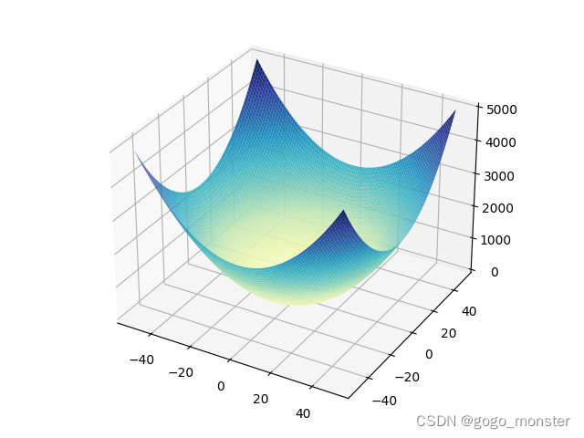
6. 通过mplot3d绘制三维图形
6.1 绘制三维曲线图
可以通过matplotlib库里的plot_surface方法来绘制三维曲线。
"""coding = utf-8"""

import numpy as np
from matplotlib import cm
import matplotlib.pyplot as plt
from mpl_toolkits.mplot3d import Axes3D

fig = plt.figure()
ax = fig.add_subplot(111, projection = '3d')
x = np.arange(-50, 51, 1)
# 通过meshgrid把数据网格化
gridX, gridY = np.meshgrid(x, x)
# 定义待绘制函数
z = gridX**2 + gridY**2
# 绘制三维曲线,rstride和cstride表示图像上行向和列向的条纹间隔,cmap表示绘制时的渐变色
ax.plot_surface(gridX, gridY, z, rstride = 1, cstride = 1, cmap = cm.YlGnBu)
plt.show()
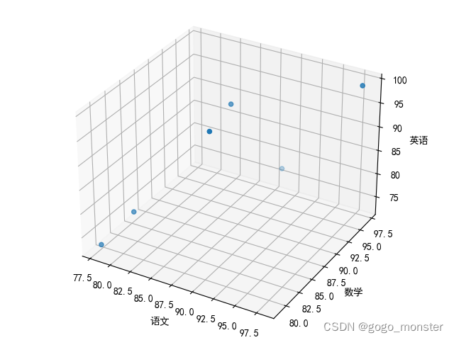
6.2 绘制三维散点图
scatter方法不仅可以绘制二维散点图的方法,还可以通过该方法绘制三维散点图。
"""coding = utf-8"""

import numpy as np
import matplotlib.pyplot as plt
from mpl_toolkits.mplot3d import Axes3D

# 分别表示语文、数学和英语的成绩
x = [98, 86, 80, 91, 78, 86]
y = [97, 91, 82, 93, 79, 87]
z = [99, 95, 78, 82, 73, 93]
# 绘制三维散点图
fig = plt.figure()
ax = Axes3D(fig)
ax.scatter(x, y, z)
# 设置中文
plt.rcParams['font.sans-serif'] = ['SimHei']
# 添加坐标轴(顺序是Z,Y,X)
ax.set_zlabel('英语')
ax.set_ylabel('数学')
ax.set_xlabel('语文')
plt.show()
6.3 绘制三维柱状图
我们可以通过bar3d方法以三维柱状图的方式直观的展示我们的案例。
"""coding = utf-8"""

import matplotlib.pyplot as plt
from mpl_toolkits.mplot3d import Axes3D

# X轴刻度
javaYears = [1, 2, 3, 4, 5]
# Y轴刻度
dbYears = [1, 2, 3, 4, 5]
# 对应的工资
salary = [6500, 8000, 10000, 12000, 15000]
fig = plt.figure()
# 设置三维坐标轴
ax = fig.add_subplot(111, projection = '3d')
# 设置标题
ax.set_title('技能和工资对照表')
plt.bar(javaYears, dbYears, zs = salary, zdir = 'zs', color = 'rgb')
# 设置中文
plt.rcParams['font.sans-serif'] = ['SimHei']
# 设置3个维度坐标轴的标签文字
ax.set_xlabel('Java工作年限')
ax.set_ylabel('数据库经验')
ax.set_zlabel('工资')
plt.show()
注:最后一段代码没有找出错误原因,图片未展示。有能够展示出来的可以和我对话,互相交流学习。


Matplotlib数据可视化&spm=1001.2101.3001.5002&articleId=123070524&d=1&t=3&u=84160d8533b647a68ce14b339851e7d6)
 1222
1222

 被折叠的 条评论
为什么被折叠?
被折叠的 条评论
为什么被折叠?
 到【灌水乐园】发言


