How is the Feature Score(Importance) in the XGBoost Package Calculated Using R?

XGBoost (Extreme Gradient Boosting) is one of the most popular machine learning algorithms due to its high performance and efficiency in handling structured data. Understanding which features contribute most to the model's predictions can be crucial, especially in real-world applications where interpretability is essential. This process is called feature importance analysis using R Programming Language.

In this article, we will explore how the XGBoost package calculates feature importance scores in R, and how to visualize and interpret them.

Step 1: Installing and Loading the XGBoost Package

First, make sure you have XGBoost and other necessary packages installed:

library(xgboost)
library(dplyr)
library(ggplot2)

Step 2: Training an XGBoost Model

Let’s start with an example dataset, the iris dataset, which is built into R.

# Load the iris dataset
data(iris)

# Convert the target variable 'Species' into a binary numerical outcome (for simplicity)
iris$Species <- as.numeric(iris$Species == "virginica")  # Binary classification: Virginica vs Non-Virginica

# Prepare the data matrices
X <- as.matrix(iris[, -5])   # Explanatory variables
y <- iris$Species            # Target variable

# Set training parameters
params <- list(
  objective = "binary:logistic",  # Binary classification
  eval_metric = "logloss",        # Evaluation metric
  eta = 0.1,                      # Learning rate
  max_depth = 3                   # Maximum depth of trees
)

# Train the XGBoost model
xgb_model <- xgboost(data = X, label = y, params = params, nrounds = 100, verbose = 0)

Step 3: Extracting Feature Importance Scores

Once you’ve trained your model, you can extract feature importance using the xgb.importance() function. This function returns a data frame containing different metrics of feature importance.

# Extract feature importance
feature_importance <- xgb.importance(model = xgb_model)
print(feature_importance)

Output:

        Feature        Gain      Cover  Frequency
1:  Petal.Width 0.590551293 0.42486643 0.35807860
2: Petal.Length 0.382338711 0.44810853 0.35807860
3:  Sepal.Width 0.023858999 0.09076455 0.19650655
4: Sepal.Length 0.003250997 0.03626048 0.08733624

The xgb.importance() function returns the following columns by default:

• Feature: The feature names
• Gain: Gain represents the improvement in accuracy (loss reduction) brought by a feature to the branches it is used in. It measures how much each feature contributes to the model's predictive power, with higher values indicating more important features.
• Cover: Cover measures the relative number of observations associated with the feature. It indicates how many times a feature is used to split data across all trees in the model.
• Frequency: Frequency is simply the percentage of times a feature appears in all trees of the model. It shows how frequently a feature is selected, which might not always correlate with its actual contribution (gain) to the model.

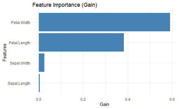
Step 4: Visualizing Feature Importance

You can visualize feature importance using xgb.plot.importance() or create a custom visualization with ggplot2.

# Custom visualization with ggplot2
feature_importance <- feature_importance %>% arrange(desc(Gain))

ggplot(feature_importance, aes(x = reorder(Feature, Gain), y = Gain)) +
  geom_bar(stat = "identity", fill = "steelblue") +
  coord_flip() +
  labs(title = "Feature Importance (Gain)", x = "Features", y = "Gain") +
  theme_minimal()

Output:

Advanced Techniques for Feature Importance Analysis

Now we will discuss Advanced Techniques for Feature Importance Analysis:

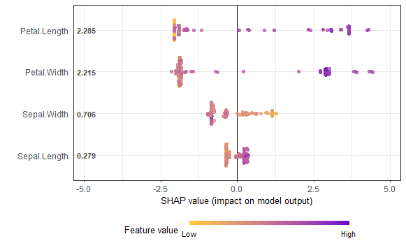
Shapley Values for Better Interpretability

Although feature importance in XGBoost is helpful, it may not always provide the full picture, especially when features interact. Shapley values offer a more accurate, game-theoretic approach to understanding feature importance. To calculate Shapley values for XGBoost, you can use the SHAPforxgboost package.

# Install SHAPforxgboost
install.packages("SHAPforxgboost")
library(SHAPforxgboost)

# Calculate SHAP values
shap_values <- shap.values(xgb_model = xgb_model, X_train = X)
shap_long <- shap.prep(shap_contrib = shap_values$shap_score, X_train = X)

# Visualize SHAP summary plot
shap.plot.summary(shap_long)

Output:

Conclusion

Feature importance scores in XGBoost provide valuable insights into which features contribute most to your model's predictions. By understanding metrics like Gain, Cover, and Frequency, you can interpret the significance of each feature. This guide demonstrated how to extract and visualize these scores in R using the xgboost package, providing you with the necessary tools to enhance your model interpretability.