Non-Negative Matrix Factorization (NMF) is a group of algorithms used in multivariate analysis and linear algebra to factorize a matrix
However scikit-learn implementation does not support missing values (NaN) in the data matrix. Due to this it requires preprocessing steps to handle any missing data before applying NMF. Before we start imputing missing values let's first visualize them to understand the problem better.
- Here we will import numpy, pandas, matplotlib and seaborn.
- Here we will create a synthetic dataset with missing values.
import numpy as np
import pandas as pd
import seaborn as sns
import matplotlib.pyplot as plt

# Creating data with missing values
np.random.seed(0)
data = np.random.rand(10, 5)
data[2, 1] = np.nan
data[5, 3] = np.nan
data[7, 2] = np.nan

df = pd.DataFrame(data, columns=[f'Feature_{i}' for i in range(data.shape[1])])

print(df)
Output:

Strategies for Handling Missing Values
1. Imputation with Zeroes
One most common approach is to replace missing values with zeroes. This method is simple but can lead to biased results because the algorithm treats these zeroes as actual data points rather than missing entries. This approach is often used when the dataset is sparse and zeroes can be considered as valid observations in some contexts such as recommendation systems.
zero_imputed = df.fillna(0)
print(zero_imputed)
Output:
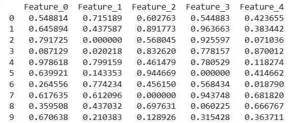
As we can see in above image all missing values are replaced with 0.
2. Mean Imputation
In mean imputation missing values are replaced with the mean of the non-missing values in the same column. This approach maintain the overall distribution of the data but can underestimate variability and led to biased estimates. It works well when the data is not highly skewed.
mean_imputed = df.fillna(df.mean())
print(mean_imputed)
Output:
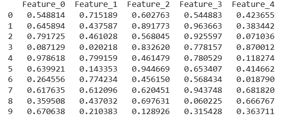
Missing values are replaced with the average value of each column.
3. Iterative Imputation
Iterative imputation is provided by scikit-learn's method called IterativeImputer. It models each feature with missing values as a function of other features and iteratively predicts the missing values. This method can capture the underlying data structure better than simple imputation techniques and is suitable for datasets where correlations exist between features.
from sklearn.experimental import enable_iterative_imputer
from sklearn.impute import IterativeImputer

imputer = IterativeImputer(max_iter=10, random_state=0)
df_imputed = imputer.fit_transform(df)
df_imputed = pd.DataFrame(df_imputed, columns=df.columns)

print("Data after Iterative Imputation:")
print(df_imputed)
Output:
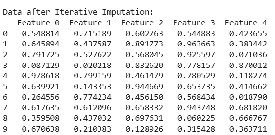
Missing values are filled by predicting them based on other features.
4. Matrix Factorization Imputation
One advanced approach to handling missing values is to use matrix factorization techniques like NMF itself for imputation. In this case NMF is applied to the incomplete matrix with missing entries and the matrix is reconstructed by factoring it into two lower-rank matrices. The missing values are predicted as part of the factorization process.
This method works well because NMF is designed to find latent patterns in the data is important.
from sklearn.decomposition import NMF

model = NMF(n_components=2, init='random', random_state=0)
W = model.fit_transform(df_imputed)
H = model.components_

data_reconstructed = np.dot(W, H)
print("Reconstructed Data from NMF:")
print(pd.DataFrame(data_reconstructed, columns=df.columns))
Output:
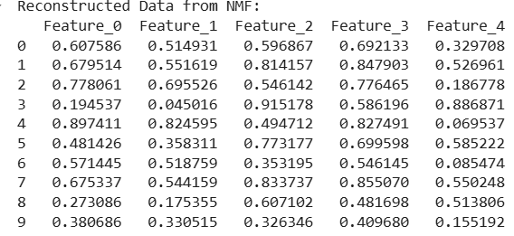
Reconstructed data is close to the imputed input. It uses patterns in the data to estimate missing values.
5. Nearest Neighbor Imputation
Another advanced technique is nearest neighbor imputation which can be used when we have additional context about the data such as similarities between rows or columns. Nearest neighbors imputation fills missing values based on the values of the nearest neighbors in the dataset. This method is useful when similar items or users exhibit similar behaviors.
from sklearn.impute import KNNImputer

imputer = KNNImputer(n_neighbors=3)
df_imputed = imputer.fit_transform(df)
print("Data after KNN imputation:")
print(pd.DataFrame(df_imputed, columns=df.columns))
Output:
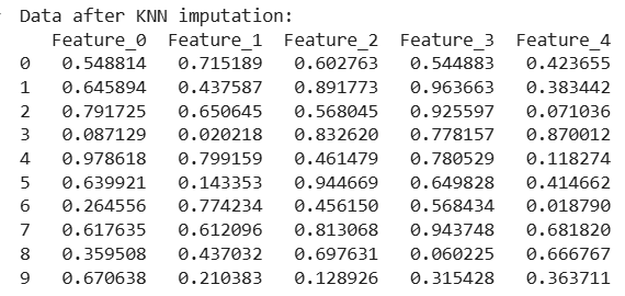
Each missing value is filled using the average of its 3 nearest rows (neighbors)
Implementing NMF After Imputation
Once the missing values are imputed we can proceed with applying NMF using scikit-learn. The below example show how to perform NMF on a dataset with imputed values:
model = NMF(n_components=2, init='random', random_state=0)
W = model.fit_transform(df_knn_imputed)
H = model.components_

data_reconstructed = np.dot(W, H)

print("\nNMF W Matrix (Features):")
print(W)
print("\nNMF H Matrix (Components):")
print(H)
print("\nReconstructed Data from NMF:")
print(pd.DataFrame(data_reconstructed, columns=df.columns))
Output:
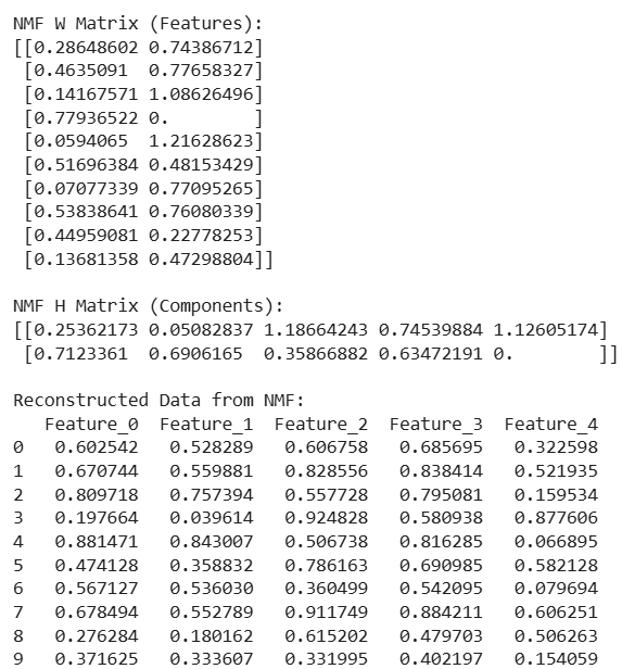
In the above output image
Evaluating the Impact of Imputation
We can check how good our imputation and factorization are using Root Mean Squared Error (RMSE). It tells how close the reconstructed matrix is to the original. Lower RMSE values indicate better reconstruction and more effective imputation.
from sklearn.metrics import mean_squared_error

def compute_rmse(original, reconstructed):
    original_df = pd.DataFrame(original, columns=df.columns)
    reconstructed_df = pd.DataFrame(reconstructed, columns=df.columns)
    original_df.fillna(0, inplace=True)
    return np.sqrt(mean_squared_error(original_df, reconstructed_df))

rmse = compute_rmse(df, data_reconstructed)
print(f'RMSE: {rmse}')
Output:
RMSE: 0.23080412343029189
In the above output the RMSE is 0.23 which shows a small difference between the original and reconstructed data. This means the imputed data and NMF reconstruction are close to the original values.
