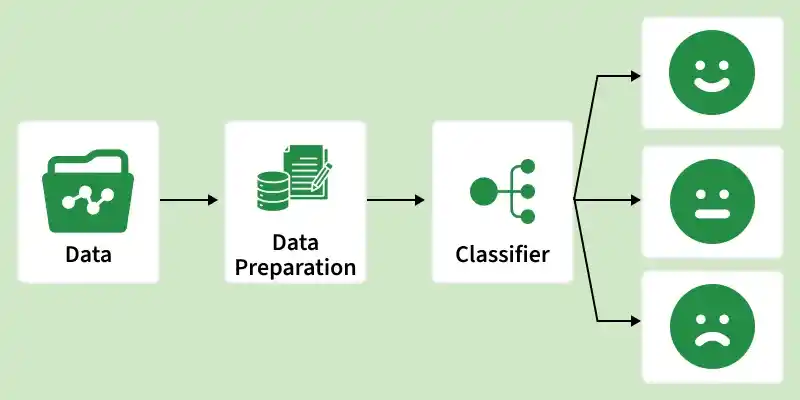
Sentiment Analysis using NLTK

Sentiment Analysis using NLTK involves analyzing text data to determine whether the expressed opinion is positive, negative or neutral. NLTK provides essential tools for text preprocessing, tokenization, and sentiment scoring, making it a popular choice for basic NLP sentiment classification tasks.

• Performs text preprocessing like tokenization and stop‑word removal
• Uses sentiment lexicons such as VADER for polarity scoring
• Commonly applied in reviews, social media analysis, and feedback systems

Implementing Sentimental Analysis using NLTK

In this section, we are going to perform sentiment analysis with NLTK using Twitter samples dataset using the following steps:

Step 1: Installing NLTK

We need to install NLTK and support packages for our model.

!pip install nltk scikit-learn matplotlib seaborn

NLTK packages:

import nltk
nltk.download('punkt', force=True)
nltk.download('stopwords', force=True)
nltk.download('wordnet', force=True)
nltk.download('vader_lexicon', force=True)
nltk.download('averaged_perceptron_tagger', force=True)
nltk.download('punkt_tab', force=True)

Step 2: Loading and Preprocessing Data

The sample documents can be downloaded from here.

For sentiment analysis:

• Loads positive and negative sentence lists from JSON files using Python’s json.load() for structured access.
• Combines and shuffles data for randomized training and testing splits, preventing bias in model training.

import json
import random
with open('positive_data.json', 'r') as f:
    positive_data = json.load(f)

with open('negative_data.json', 'r') as f:
    negative_data = json.load(f)

data = positive_data + negative_data
random.shuffle(data)

print(f"Total samples loaded: {len(data)}")

Output:

Total samples loaded: 196

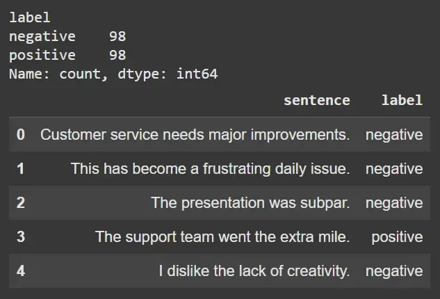
Step 3: Explore Data Analysis (EDA)

Quick look at data distribution:

• Uses pandas to visualize and count label distribution for data balance.
• Displays sample entries to inspect text format and sentiment labeling.

import pandas as pd

df = pd.DataFrame(data)
print(df['label'].value_counts())

df.head()

Output:

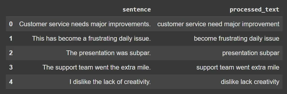
Step 4: Text Preprocessing Pipeline

• Defines a function to tokenize sentences into words with word_tokenize.
• Converts words to lowercase, removes stop words and punctuation for noise reduction.
• Lemmatizes tokens using WordNetLemmatizer to reduce inflectional forms to base words.
• Applies preprocessing to all sentences, producing cleaned text for feature extraction.

from nltk.tokenize import word_tokenize
from nltk.corpus import stopwords
from nltk.stem import WordNetLemmatizer
import string

stop_words = set(stopwords.words('english'))
lemmatizer = WordNetLemmatizer()


def preprocess_text(text):
    tokens = word_tokenize(text)
    filtered_tokens = [w.lower() for w in tokens if w.isalpha()
                       and w.lower() not in stop_words]

    lemmas = [lemmatizer.lemmatize(token) for token in filtered_tokens]
    return ' '.join(lemmas)


df['processed_text'] = df['sentence'].apply(preprocess_text)
print(df[['sentence', 'processed_text']].head())

Output:

Step 5: Feature Extraction

• Transforms processed text into numerical vectors using CountVectorizer creating a word occurrence matrix also known as Bag of Words.
• Maps sentiment labels to binary values (positive = 1, negative = 0) for model compatibility.
• Outputs matrix shape for verifying feature dimensionality.

from sklearn.feature_extraction.text import CountVectorizer

vectorizer = CountVectorizer()
X = vectorizer.fit_transform(df['processed_text'])
y = df['label'].map({'positive': 1, 'negative': 0}).values

print(f"Feature matrix shape: {X.shape}")

Output:

Feature matrix shape: (196, 347)

Step 6: Train-Test Split

We will:

• Splits features and labels into training and test sets with train_test_split, preserving class proportions (stratify).
• Enables objective model evaluation.

from sklearn.model_selection import train_test_split

X_train, X_test, y_train, y_test = train_test_split(
    X, y, test_size=0.2, random_state=42, stratify=y
)

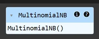
Step 7: Model Training

Use Multinomial Naive Bayes:

• Trains a MultinomialNB classifier, which is efficient for word frequency-based text data.
• Fits the model on training data to learn text-sentiment relationships.

from sklearn.naive_bayes import MultinomialNB

model = MultinomialNB()
model.fit(X_train, y_train)

Output:

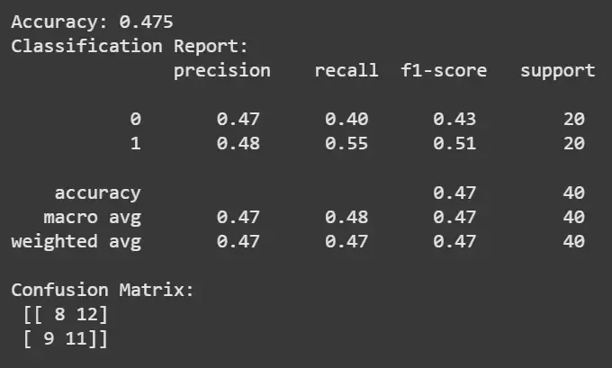
Step 8: Model Evaluation

• Predicts sentiments on the test set and computes accuracy score.
• Prints classification report detailing precision, recall and F1-score for each class.
• Generates confusion matrix to visualize prediction correctness and misclassifications.

from sklearn.metrics import accuracy_score, classification_report, confusion_matrix

y_pred = model.predict(X_test)

print("Accuracy:", accuracy_score(y_test, y_pred))
print("Classification Report:\n", classification_report(y_test, y_pred))

cm = confusion_matrix(y_test, y_pred)
print("Confusion Matrix:\n", cm)

Output:

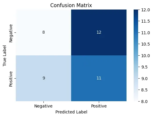
Step 9: Visualization of Confusion Matrix

We will visualize the confusion matrix:

• Use matplotlib and seaborn to plot a heatmap for the confusion matrix.
• Visualizes true vs predicted labels for diagnostic insights.

import matplotlib.pyplot as plt
import seaborn as sns

plt.figure(figsize=(6, 4))
sns.heatmap(cm, annot=True, fmt='d', cmap='Blues', xticklabels=[
            'Negative', 'Positive'], yticklabels=['Negative', 'Positive'])
plt.xlabel("Predicted Label")
plt.ylabel("True Label")
plt.title("Confusion Matrix")
plt.show()

Output:

Step 10: Use NLTK’s VADER Sentiment Analyzer (Lexicon-based)

Here:

• Instantiates SentimentIntensityAnalyzer to compute sentiment polarity.
• Defines a function returning 'positive', 'negative', or 'neutral' based on the compound score.
• Applies VADER to example and dataset sentences to compare lexicon-based vs ML-based approaches.

from nltk.sentiment import SentimentIntensityAnalyzer

sia = SentimentIntensityAnalyzer()


def get_vader_sentiment(text):
    scores = sia.polarity_scores(text)
    compound = scores['compound']
    if compound >= 0.05:
        return 'positive'
    elif compound <= -0.05:
        return 'negative'
    else:
        return 'neutral'


sample_text = "I love this product! It's amazing."
print(get_vader_sentiment(sample_text))

df['vader_sentiment'] = df['sentence'].apply(get_vader_sentiment)
print(df[['sentence', 'vader_sentiment']].head())

Output:

Positive

Step 11: Compare VADER and ML Model Predictions

• Maps VADER sentiment outputs to binary for accuracy comparison against labels.
• Calculates and prints VADER-based accuracy for benchmark evaluation.

from sklearn.metrics import accuracy_score

df['vader_sentiment'] = df['sentence'].apply(get_vader_sentiment)

vader_labels = df['vader_sentiment'].map(
    {'positive': 1, 'negative': 0, 'neutral': -1})
valid_indices = vader_labels != -1

print("VADER Sentiment Accuracy compared to labels:")
print(accuracy_score(y[valid_indices], vader_labels[valid_indices]))

Output:

VADER Sentiment Accuracy compared to labels:
0.9548387096774194

Step 12: Predict Results on New Sentences

We will predict the results of more sentences using the model,

• Preprocesses new input sentences and predicts sentiment using the trained model.
• Demonstrates real-world use for unseen text.

def predict_sentiment(text):
    processed = preprocess_text(text)
    vectorized = vectorizer.transform([processed])
    pred = model.predict(vectorized)[0]
    return 'positive' if pred == 1 else 'negative'


test_sentences = [
    "This is an amazing product with great quality.",
    "I did not like the service at all, very poor."
]

for text in test_sentences:
    print(f"Sentence: {text} => Sentiment: {predict_sentiment(text)}")

Output:

Sentence: This is an amazing product with great quality.
=> Sentiment: positive

Sentence: I did not like the service at all, very poor.
=> Sentiment: negative

As we can see the model was able to predict whether it was positive or negative emotion.

Step 13: Save the Model and Vectorizer

Here:

• Serializes the trained model and vectorizer with joblib.dump, enabling future predictions without retraining.
• Facilitates deployment and reproducibility.

import joblib

joblib.dump(model, 'sentiment_nb_model.joblib')
joblib.dump(vectorizer, 'count_vectorizer.joblib')

Output:

['count_vectorizer.joblib']