A Control Chart is a statistical chart used to monitor process performance over time and identify variations that fall outside acceptable limits. It helps distinguish between normal variation and special-cause variation by using upper and lower control limits. They are useful for:
- Identifying outliers and abnormal trends
- Monitoring the stability of a process over time
- Understanding variation using standard deviation
- Visualizing upper and lower control limits
- Supporting data-driven decision-making
Creating a Control Chart
Tableau does not provide a direct Control Chart option, but it can be created using table calculations, parameters and a dual-axis setup.
Note: For this article, a sample dataset "vgsales.csv" is used, to download click here.
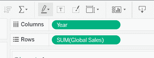
Step 1: Create the Base Line Chart
Drag the Year field to the Columns shelf and drag Global_Sales to the Rows shelf.
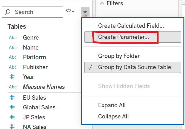
Step 2: Create Parameter for Standard Deviation Level
1. Click the drop-down arrow in the Data pane and select Create Parameter.
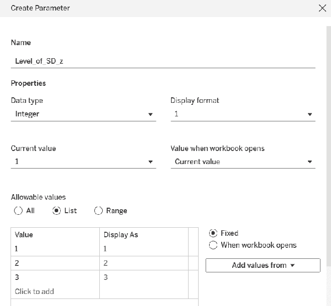
2. Configure the parameter as follows:
- Name: Level_of_SD_z
- Data Type: Integer
- Allowable Values: List
- List of Values: 1, 2, 3
- Click OK.
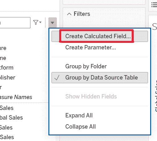
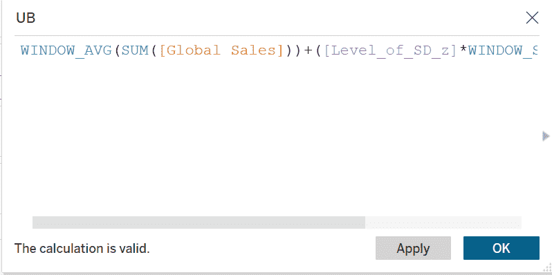
Step 3: Create Upper Bound (UB)
1. From the Data pane drop-down, select Create Calculated Field and name the field UB.
2. Enter the following formula:
WINDOW_AVG( SUM( [Global_Sales] ) ) + ( [Level_of_SD_z] * WINDOW_STDEV( SUM( [Global_Sales] ) ) )
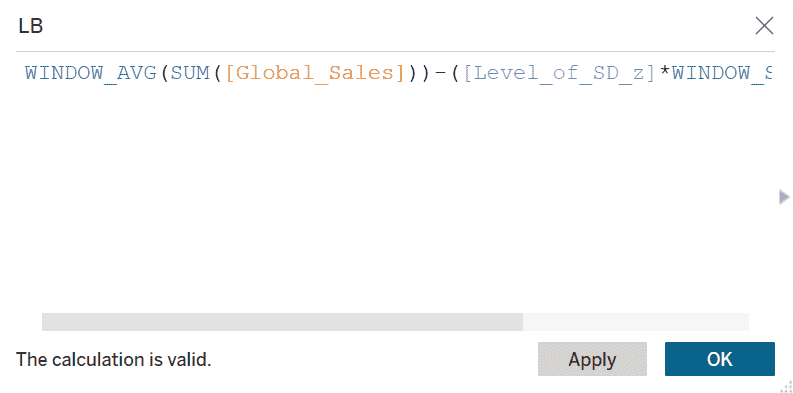
Step 4: Create Lower Bound (LB)
Again select Create Calculated Field and name the field LB. Enter the following formula:
WINDOW_AVG( SUM( [Global_Sales] ) ) - ( [Level_of_SD_z] * WINDOW_STDEV( SUM( [Global_Sales] ) ) )
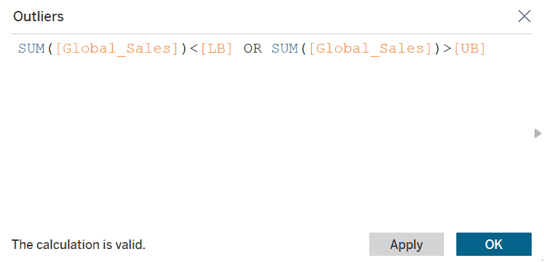
Step 5: Identify Outliers
Create another calculated field and name it Outliers and enter the following condition:
SUM( [Global_Sales] ) < [LB] OR SUM( [Global_Sales] ) > [UB]
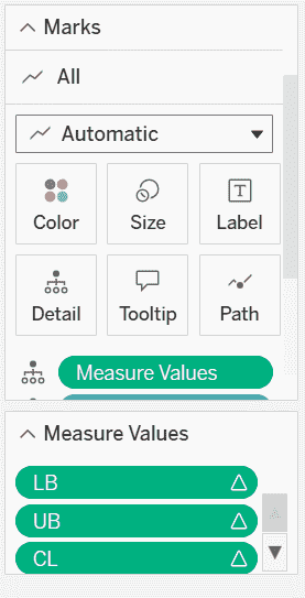
Step 6: Configure Measure Values
Drag Measure Values to the Marks card and in the Measure Values shelf, keep only LB and UB
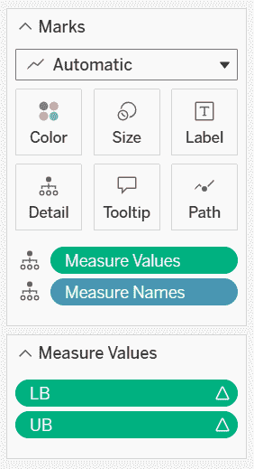
Remove all other measures.
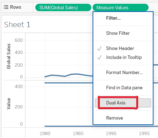
Step 7: Create Dual Axis
Drag Measure Values to the Rows shelf and right-click the second axis and select Dual Axis.
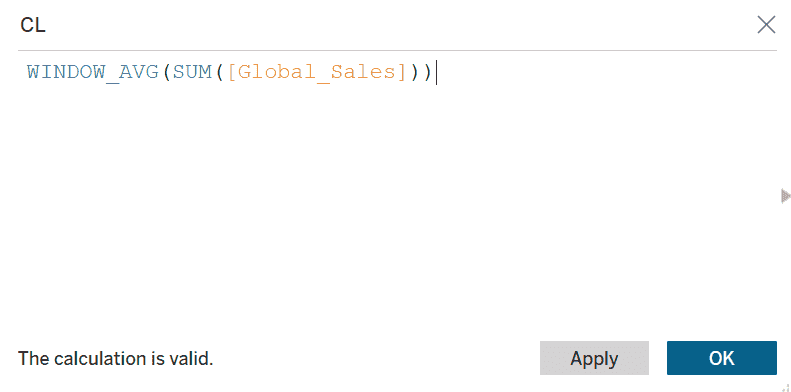
Step 8: Add Central Line (CL)
Create a new calculated field named CL and enter the formula:
WINDOW_AVG( SUM( [Global_Sales] ) )
Drag CL into Measure Values.
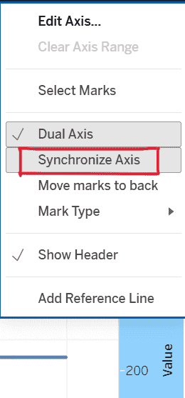
Step 9: Synchronize Axes
Right-click on the Value axis and select Synchronize Axis.
Step 10: Highlight Outliers
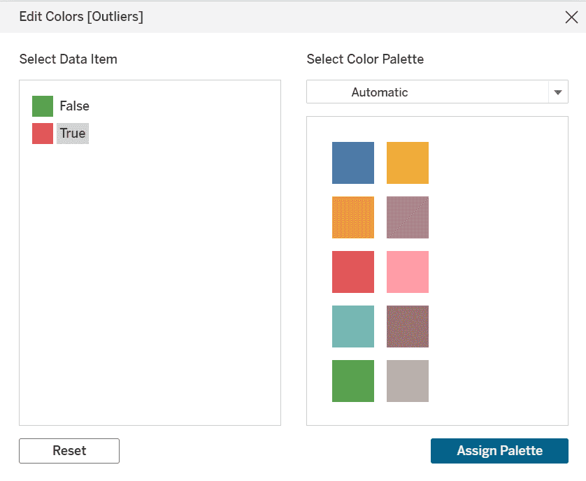
1. In the Global_Sales Marks card, drag Outliers to the Color shelf.
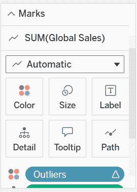
2. Click Edit colors: False -> Green and True -> Red.
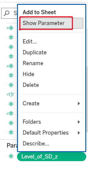
Step 11: Show Parameter Control
Go to the Parameters pane right-click Level_of_SD_z and select Show Parameter.
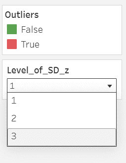
Step 12: Adjust Control Limits
Change the Level_of_SD_z value to:
- 1 for tighter limits
- 2 for moderate limits
- 3 for wider limits
Final Output
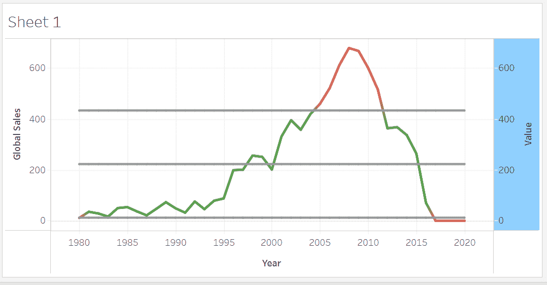
The final Control Chart displays:
- A central average line (CL)
- Upper and lower control limits (UB & LB)
- Sales trends over time
- Outliers highlighted clearly in red
- Interactive control using standard deviation levels
This chart is ideal for monitoring stability, detecting anomalies and analyzing process behavior over time.
